1. Overview
Algorithmic complexity is a measure of the resources an algorithm requires with respect to its input size. The two main types of complexity are time complexity and space complexity. Furthermore, time complexity refers to the number of operations performed by an algorithm, whereas space complexity refers to the amount of memory consumed. Furthermore, understanding these complexities is essential for evaluating an algorithm’s efficiency and enhancing software systems.
In this tutorial, we’ll look at how to analyze an algorithm’s complexity. Additionally, we’ll talk about time and space complexity, as well as practical ways to evaluate them.
2. Time Complexity
The size of the input measures the time complexity of an algorithm. Additionally, it’s commonly expressed in Big-O notation.
2.1. Constant Time O(1)
Constant time complexity, also known as O(1), refers to operations that take the same amount of time regardless of input size. Moreover, these operations are very efficient and unaffected by larger data sets.
2.2. Linear Time O(n)
Linear time complexity, also known as O(n), occurs in algorithms that analyze each input element exactly once, such as linear search, which is straightforward but can become inefficient with bigger data sets.
2.3. Polynomial Time O(n^m)
Nested loops cause polynomial complexity in algorithms. Furthermore, each loop processes the input, increasing execution time as the input size grows.
2.4. Logarithmic Time O(log n)
Divide and conquer algorithms, such as binary search, have a logarithmic complexity. Moreover, these algorithms drastically reduce the size of the problem with each step, making them suitable for large datasets.
2.5. Factors Affecting Time Complexity
The amount of the input data is one factor that affects time complexity, as it directly affects the number of operations required: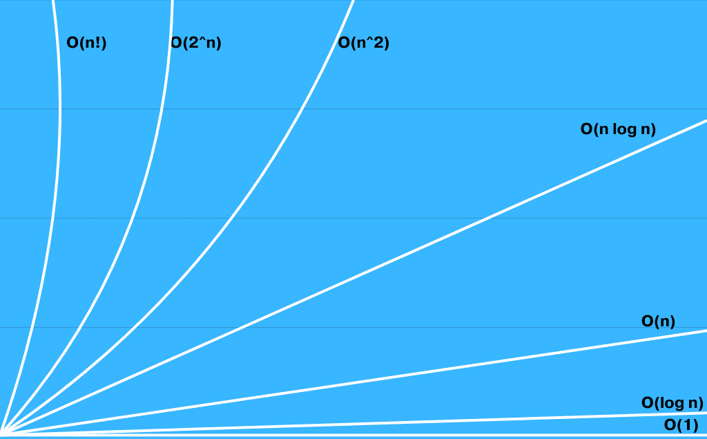
In this graph, we show the growth rates of common time complexities. Constant time O(1) remains constant regardless of input size, but exponential time O(2^n) rises rapidly and becomes infeasible for even small input sizes. Finally, linear O(n), quadratic O(n^2), and other complexities fall in the middle, with logarithmic O(log n) being particularly efficient for bigger datasets.
3. Space Complexity
Space complexity measures how much memory an algorithm requires for the size of its input.
3.1. Constant Space Complexity
Constant space algorithms require a given amount of memory, regardless of input size. For example, exchanging two variables takes O(1) space.
3.2. Linear Space Complexity
Linear space algorithms release memory in proportion to the input size. Thus, it’s common in algorithms that keep or process every element of the input.
3.3. Logarithmic Space Complexity
Algorithms having logarithmic space complexity are frequently seen in recursive techniques, where the recursion depth determines memory usage.
3.4. Quadratic Space Complexity
Certain algorithms can require a memory matrix or similar data structures in a quadratic space complexity, Hence, memory usage is proportional to the square of the input size.
4. Evaluating Time Complexity
Evaluating an algorithm’s time complexity is figuring out how long it takes to execute as the size of the input increases.
4.1. Analyzing Loops
Loops directly increase time complexity and are an essential component of many algorithms. Because each iteration adds a fixed amount of work, the time complexity for a single loop that iterates n times is O(n):
def linear_loop(arr):
    for num in arr:
        print(num)
In this example, the function iterates through each element of the array*,* because the loop runs n times, its time complexity is O(n).
Furthermore, let’s look at nested loops and how to evaluate them:
def quadratic_loop(arr):
    for i in arr:
        for j in arr:
            print(i, j)
In this example, the outer loop is executed n times, and the inner loop is executed n times for each iteration, this results in O(n^2) complexity.
The following is a further example of a polynomial time algorithm with an O(n^3) complexity:
def cubic_loop(arr):
    for i in arr:
        for j in arr:
            for k in arr:
                print(i, j, k)
In this example, the complexity is O(n^3) due to the three nested loops that iterate n times each, totaling n × n × n = n^3.
In conclusion, the complexity increases with the number of nested loops. A double loop has O(n^2) complexity when both loops iterate n times. Likewise, O(n^3) is given for a triple nested loop. Furthermore, finding the number of nesting layers and observing how the number of iterations varies with the size of the input are crucial steps in identifying loop-related complexities.
4.2. Evaluating Recursive Calls
The complexity of recursive algorithms can be different based on how the problem size evolves with each call. Additionally, the complexity is O(log n) if the input size is decreased by a fixed amount (for example, half), as is the case with algorithms such as binary search:
def binary_search(arr, target, low, high):
    if low > high:
        return -1
    mid = (low + high)
    if arr[mid] == target:
        return mid
    elif arr[mid] < target:
        return binary_search(arr, target, mid + 1, high)
    else:
        return binary_search(arr, target, low, mid - 1)
In this example, each recursive call reduces the input size by half. Furthermore, for an array of size n, the maximum number of calls is log(n), giving O(log n) complexity.
Furthermore, let’s consider other similar examples:
def factorial(n):
    if n == 0:
        return 1
    return n * factorial(n - 1)
Here, the factorial function makes n recursive calls, each of which reduces the problem size by 1. Hence, this results in a complexity of O(n).
Furthermore, the complexity of divide and conquer algorithms, such as merge sort, *which split and recombine data, is determined by recurrence relations and frequently yields O(n log n):*
def merge_sort(arr):
    if len(arr) > 1:
        mid = len(arr)
        left = arr[:mid]
        right = arr[mid:]
        merge_sort(left)
        merge_sort(right)
In this example, we split the input into two halves log n, and combine them in linear time O(n). Thus, the whole complexity equals O(n log n).
4.3. Constant Time Operations
The complexity of constant time operations, like simple arithmetic or single-element access in an array, is O(1):
def constant_time_operations(arr):
    print(arr[0])
    print(len(arr))
    print(arr[0] + arr[1])
In this example, these operations take a fixed amount of time regardless of input size. For example, accessing the first entry of a list, performing arithmetic operations, and determining the length of an array are all O(1).
In conclusion, these operations are simple to recognize because they don’t depend on the input size. Additionally, In small operations, they dominate the complexity, but in big algorithms, they are usually insignificant when compared to loops or recursion.
5. Evaluating Space Complexity
The memory needed by an algorithm as a function of input size is measured by space complexity.
5.1. Fixed and Variable Memory Usage
Constants, program instructions, and static variables are examples of fixed memory consumption that contribute to O(1) complexity because they don’t change with input size:
def swap(a, b):
    temp = a
    a = b
    b = temp
In this example, the swap function allocates a fixed amount of memory to the variables a, b, and temp. Thus, the space complexity is O(1) because the memory usage is unaffected by the input size.
Furthermore, arrays and dynamically allocated structures are examples of variable memory usage that increases with input size. For instance, O(n) space is needed to store n elements in an array:
def copy_array(arr):
    copy = [0] * len(arr)
    for i in range(len(arr)):
        copy[i] = arr[i]
    return copy
In this example, the copy_array function generates a new list copy with the same size as the input list arr. Additionally, because the memory usage increases with input size n, the space complexity is O(n).
5.2. Analyzing Auxiliary Space
Auxiliary space is the temporary memory needed by an algorithm. Additionally, O(n) auxiliary space is used in sorting algorithms like merge sort, which combines additional arrays:
def merge_sort(arr):
    if len(arr) > 1:
        mid = len(arr)
        left = arr[:mid]
        right = arr[mid:]
        merge_sort(left)
        merge_sort(right)
In this example, merge sort takes advantage of extra memory to store the separated subarrays (left and right). Thus, the total auxiliary space required is proportional to the input size n, hence the space complexity is O(n).
Furthermore, let’s consider other sorting algorithms:
def quicksort(arr, low, high):
    if low < high:
        pivot_index = partition(arr, low, high)
        quicksort(arr, low, pivot_index - 1)
        quicksort(arr, pivot_index + 1, high)
In this example, quicksort performs recursion using the call stack. Thus, the recursion depth is logarithmic log n, and the auxiliary space complexity is O(log n).
However, quicksort and other sorting algorithms only need O(log n) space for the recursion stack. Additionally, we can keep track of the temporary structures produced during execution to calculate auxiliary space.
5.3. Evaluating Recursive Space Usage
Memory usage of recursive algorithms on the call stack is proportional to the depth of recursion. Additionally, a recursive algorithm with n layers of recursion, for instance, needs O(n) stack space:
def binary_search_recursive(arr, target, low, high):
    if low > high:
        return -1
    mid = (low + high)
    if arr[mid] == target:
        return mid
    elif arr[mid] < target:
        return binary_search_recursive(arr, target, mid + 1, high)
    else:
        return binary_search_recursive(arr, target, low, mid - 1)
In this example, binary search reduces the problem size by half with each recursive call. Thus, the greatest recursion depth is log(n), with a space complexity of O(log n).
Furthermore, let’s consider other similar examples:
def factorial(n):
    if n == 0:
        return 1
    return n * factorial(n - 1)
In this example, the factorial function performs n recursive calls, each adding a new layer to the call stack. Hence, it yields a space complexity of O(n).
Moreover, the space complexity becomes O(log n) if the recursion reduces the input size exponentially. Thus, the amount of stack space needed can be calculated by looking at the depth and organization of recursive calls.
6. Conclusion
Analyzing algorithm complexity is essential for developing efficient systems. Time complexity measures the increase in execution time, whereas space complexity quantifies memory usage.
In this article, we discussed time and space complexity, explaining both concepts and practical ways to find the time and space complexity of an algorithm.
Finally, mastering these analysis can help us develop algorithms that successfully balance performance and resource utilization.