Computer Vision: 1*1 Convolution

1. Introduction

In this tutorial, we’ll discuss 1*1 convolution, a key concept in deep learning. 1*1 convolution plays an essential role in convolutional neural networks (CNNs), allowing for efficient feature extraction and dimensionality reduction.

2. What Is 1*1 Convolution?

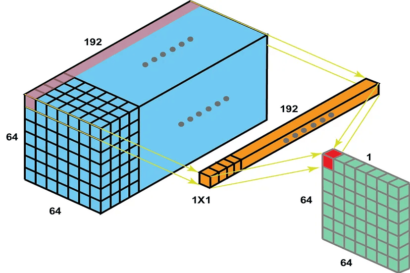
1*1 convolution (pointwise convolution) is a type of convolution operation in convolutional neural networks (CNNs). It uses a filter with a size of 1*1. This filter processes each pixel of the input data individually. It helps to reduce the number of parameters and computations. It also allows the network to learn more complex features:

3. Benefits of 1*1 Convolution

One of the primary advantages of 1*1 convolution is its ability to reduce the dimensionality of the input data. By applying a 1*1 filter, the number of channels can be decreased, effectively compressing the feature maps and lowering the computational complexity of the network. This dimensionality reduction is particularly valuable in deep learning models, where managing the size and complexity of data is crucial for efficient processing.

Additionally, 1*1 convolution facilitates the recombination of features from different channels. This process enables the creation of more complex and meaningful representations of the input data, as previously isolated features can be combined to capture more intricate patterns and relationships. This ability to recompose features adds a layer of flexibility and power to neural network architectures.

Moreover, 1*1 convolution is computationally efficient. Since it operates on individual pixels rather than larger regions, it requires less computational power compared to larger filters. This efficiency is beneficial when designing neural networks that need to balance performance with resource constraints, making 1×1 convolution a valuable tool in optimizing modern deep learning models.

4. How to Perform 1*1 Convolution

Let’s discuss how to perform 1*1 Convolution using a step-by-step guide.

4.1. Input Data Preparation (Input Tensor)

We start with an input tensor of shape (H, W, C), where H represents height, W represents width, and C represents the number of channels.

For example, suppose we have an input tensor of shape (3, 3, 2), which is a 3×3 image with 2 channels.

Let’s consider a simple example to illustrate the process of 1*1 convolution:

input_tensor = [
    [[1, 2], [3, 4], [5, 6]],
    [[7, 8], [9, 10], [11, 12]],
    [[13, 14], [15, 16], [17, 18]]
]

4.2. Define the 1*1 Filter

Next, we define a 1*1 filter of shape (1, 1, C, F), where F is the number of output channels. Each filter has a size of 1×1 and is applied to each channel of the input tensor.

For instance, we define a 1*1 filter of shape (1, 1, 2, 1), indicating one filter applied across two channels:

filter = [
    [[1, 2]]
]

4.3. Convolution Operation

To perform the convolution, for each pixel location (x, y), we multiply the values in the filter by the corresponding values in the input tensor and then sum the results. The correct operation for each pixel should look like this:

1. For the first pixel , the operation is    
2. Subsequently for  the second pixel , the operation is    
3. For the third pixel , the operation is     and similarly for the remaining pixels

4.4. Output Tensor

Finally, the output of the 1*1 convolution will be a tensor of shape (H, W, F), where F is the number of output channels.

In our example, after applying the convolution operation to each pixel in the input tensor, the output tensor would be:

output_tensor = [
    [[5], [11], [17]],
    [[23], [29], [35]],
    [[41], [47], [53]]
]

In this example, the output tensor has a shape of (3, 3, 1), indicating that the number of channels has been reduced from 2 to 1.

5. Applications of 1*1 Convolution

5.1. Network-in-Network (NiN)

The Network-in-Network (NiN) architecture is one of the early applications of 1*1 convolution. NiN uses 1*1 convolutions to increase the depth of the network without significantly increasing the number of parameters. This allows the network to learn more complex representations of the input data.

5.2. GoogLeNet (Inception Module)

GoogLeNet, also known as the Inception network, uses 1*1 convolutions in its Inception modules. The Inception module combines filters of different sizes (1*1, 3*3, 5*5) to capture features at multiple scales. The 1*1 convolutions are used to reduce the dimensionality of the input data before applying larger filters, which helps in reducing computational complexity.

5.3. Residual Networks (ResNet)

Residual Networks (ResNet) also make use of 1*1 convolutions in their bottleneck blocks. The bottleneck block consists of a sequence of 1*1, 3×3, and 1*1 convolutions. The first 1*1 convolution reduces the number of channels, the 3*3 convolution captures spatial features, and the final 1*1 convolution restores the number of channels. This design helps in reducing the computational cost while maintaining the network’s ability to learn complex features.

5.4. Implementation in Popular Deep Learning Frameworks

In TensorFlow, 1*1 convolution can be implemented using the tf.nn.conv2d function. Here’s a simple example:

import tensorflow as tf
# Input tensor of shape (batch_size, height, width, channels)
input_tensor = tf.random.normal([1, 3, 3, 2])
# 1*1 filter of shape (filter_height, filter_width, in_channels, out_channels)
filter = tf.constant([[[[1, 2]]]], dtype=tf.float32)
# Perform 1*1 convolution
output_tensor = tf.nn.conv2d(input_tensor, filter, strides=[1, 1, 1, 1], padding='VALID')
print(output_tensor)

In PyTorch, 1*1 convolution can be implemented using the torch.nn.Conv2d class. Here’s a simple example:

import torch
import torch.nn as nn
# Input tensor of shape (batch_size, channels, height, width)
input_tensor = torch.randn(1, 2, 3, 3)
# Define a 1*1 convolution layer
conv_layer = nn.Conv2d(in_channels=2, out_channels=1, kernel_size=1)
# Perform 1*1 convolution
output_tensor = conv_layer(input_tensor)
print(output_tensor)

6. Conclusion

In this article, we discussed 1*1 convolution, a powerful tool in the arsenal of convolutional neural networks. Its ability to reduce dimensionality, recombine features, and improve computational efficiency makes it a valuable addition to various network architectures. By understanding the mechanics of 1*1 convolution and its applications, we can grasp this technique to design more effective and efficient deep learning models.

Additionally, whether we’re working with TensorFlow, PyTorch, or any other deep learning framework, the principles of 1*1 convolution remain consistent and can be easily implemented to enhance our models.