How to Sample a Uniform Random Point from a Circle?

1. Introduction

In this tutorial, we’ll show how to sample a point from a uniform distribution defined over a circle.

We’ll explain how to derive the sampling distribution explicitly and how to avoid math using rejection sampling.

2. Problem Statement

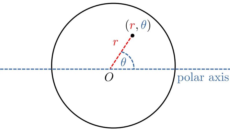
In the polar coordinate system, we define a point by its distance to the origin and the angle $\theta$ from the polar axis:

Let be the circle’s radius. Since we want to sample uniformly from the circle, the sampling density should have constant values for all $(r, \theta) \in [0, R]\times [0, 2\pi]$ :

$[(\exists c > 0)(\forall r \in [0, R])(\forall \theta \in [0, 2\pi]) f(r, \theta) = c]$

3. Incorrect Naive Solution

The first approach we might try is to sample $\theta$ uniformly from $[0, 2\pi]$ and from [0, R] :

algorithm NaiveSampling(R):
    // INPUT
    //   R = the radius of the corcle
    // OUTPUT
    //   theta, r = the polar coordinates of the sampled point
    
    theta <- uniform(0, 2 * pi)
    r <- uniform(0, R)

    return theta, r

However, this doesn’t result in a uniform distribution. To show that, let’s generate 10,000 points from a unit circle ( R=1 ):

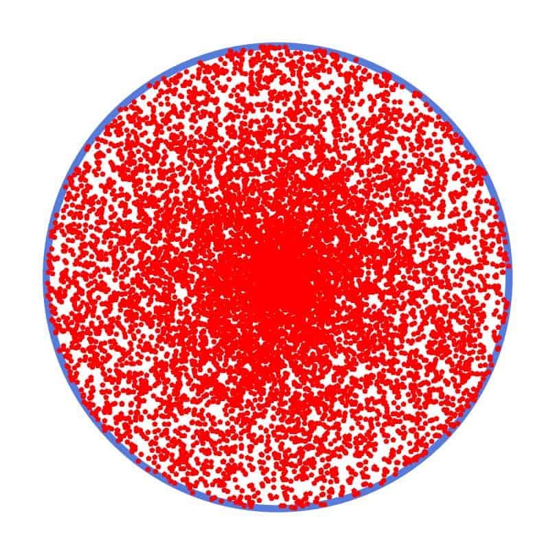
The area near the origin is more densely populated. Why?

Let’s observe that infinitely many concentric circles are inside our target circle. Since $\theta$ is uniform over $[0, 2\pi]$ , all the angles are equally likely for any radius . However, the concentric circles don’t have the same circumference, as the closer ones to the origin are smaller:

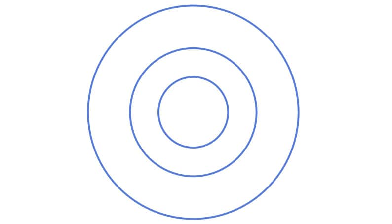
Informally, we’re covering all these concentric circles with the same number of points, but since the outer ones are larger, they have a lower sampling density, which is why this approach doesn’t work.

4. Correct Density for Radius

We must sample so that greater is more likely to be sampled.

In particular, the probability of sampling a point from an area corresponding to the point’s distance to the origin must be proportional to that area, i.e., to the area $r^2 \pi$ of the circle whose radius is . In other words, the probability of sampling from a circle with radius $r \leq R$ is the ratio of $r^2 \pi$ and the total area $R^2 \pi$ :

$[\frac{r^2 \pi}{R^2 \pi} = \frac{r^2}{R^2}]$

Intuitively, sampling from any two concentric circles (defined by their radii) should be equally likely, so the probabilities r^2 / R^2 (also defined by the radius ) should follow a uniform distribution over [0, 1] . More formally, since sampling from a circle with radius means that the sampled point can be at any distance $\leq r$ from the origin, the probability is a cumulative distribution function of a distribution over . By the probability integral transform, it’s a uniform random variable over [0, 1] .

From there, if is a random number from [0, 1] , we get by setting r^2 / R^2 = u and solving for :

$[\frac{r^2}{R^2} = u \implies r^2 = u R^2 \implies r = R \sqrt{u}]$

So, sampling $\theta$ stays the same as in the naive approach, but not for :

algorithm CorrectExplicitSampling(R):
    // INPUT
    //   R = the radius of the corcle
    // OUTPUT
    //   theta, r = the polar coordinates of the sampled point
    
    theta <- uniform(0, 2 * pi)
    r <- sqrt(uniform(0, 1)) * R

    return theta, r

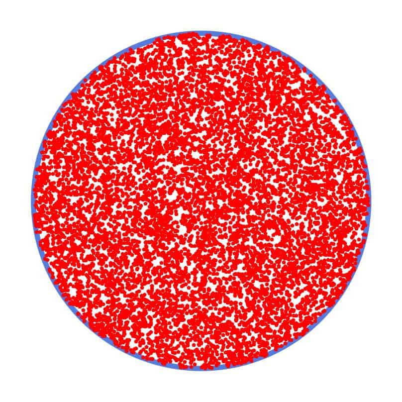
Now, the density is truly uniform over our entire circle:

5. Less Math: Rejection Sampling

If we want to sample uniformly from any geometric shape, rejection sampling offers a simple and intuitive approach that avoids explicitly dealing with probabilities and densities.

The first step is to place a shape from which we can easily sample uniform points over our target shape. In most cases, this reference shape will be a square. So, we inscribe our target circle with radius into a square whose sides have length :

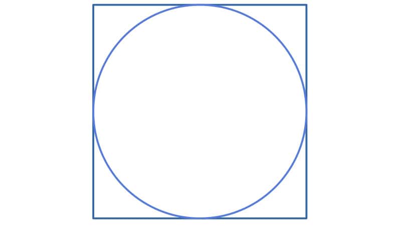
Then, we sample a point from the square. If the sampled point is in the circle, we return it (after transforming from the Cartesian to polar coordinates). Otherwise, we repeat the sampling:

algorithm RejectionSampling(x0, y0, R):
    // INPUT
    //    x0, y0 = the coordinates of the origin of the circle
    //    R = the radius of the circle
    // OUTPUT
    //    theta, r = the polar coordinates of a point inside the circle
    
    R2 <- R * R
    while true:
        // uniformly sample a point in the square
        x <- uniform(x0 - R, x0 + R)
        y <- uniform(y0 - R, y0 + R)
        
        // compute its squared distance to the center
        r2 <- (x0 - x)**2 + (y0-y)**2
        
        // check if the point is in the circle
        if r2 <= R2:
            // convert to polar coordinates
            theta <- atan2(y, x)
            r <- sqrt(r2)
    
            return theta, r

For efficiency, we compute the polar coordinates only if the point is in the circle and compare r^2 to R^2 instead of to to avoid calculating the square root if the point isn’t in the circle.

Why does this approach work? Since we cover our circle with a square of constant density, the density over the circle will also be uniform:

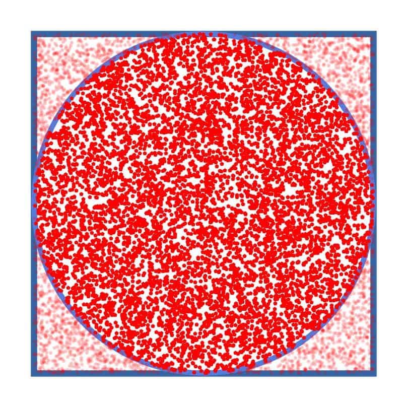
A drawback of rejection sampling is that some points fall outside the circle. The probability of sampling such a point is:

$[\frac{4R^2-R^2\pi}{4R^2}=\frac{4-\pi}{4} \approx 21.46\%]$

However, this approach is fast and straightforward to implement.

6. Conclusion

In this article, we showed how to randomly generate a point from a circle.

We can derive the sampling distribution mathematically and draw from it explicitly or use rejection sampling. Both approaches work, but the latter involves less math.

Persistence

REST

Security