Introduction to Binomial Distribution

1. Introduction

In this tutorial, we’ll discuss the binomial distribution and its application.

2. What Is Probability

Probability measures how likely an event is to occur. We use it in everyday conversations, like saying, “There’s a good chance it will rain today”, or “The odds of winning the football game is very low”.

In mathematical terms, probability is the ratio of the number of favorable outcomes to the total number of possible outcomes. For example, when we flip a fair coin, there are two possible outcomes: heads or tails. The probability of getting heads, denoted as $P(\text{heads})$ , is:

$[ P(\text{heads}) = \frac{\text{Number of favorable outcomes}}{\text{Total number of possible outcomes}} = \frac{1}{2} ]$

3. Understanding Probability Distributions

In probability, we often deal with two types of random variables: discrete and continuous. Discrete random variables take countable values, and their probabilities are described using the Probability Mass Function (PMF). This tells us the likelihood of specific outcomes, like getting a certain number of heads when flipping a coin. Continuous random variables, which can take any value within a range, use the Probability Density Function (PDF) to describe how likely the variable falls within a particular interval.

Finally, the Cumulative Distribution Function (CDF) gives us the probability that a variable is less than or equal to a certain value. It can be applied to discrete and continuous distributions.

Regarding standard distributions, discrete distributions like the Binomial, Poisson, and Geometric distributions help us understand events that we can count, while continuous ones like the Normal, Exponential, and Uniform distributions handle measurements. Since our main focus here is the Binomial distribution, we’ll dive into that next.

4. Bernoulli Trials, Precursor to the Binomial Distribution

Before diving into the binomial distribution, let’s quickly touch on Bernoulli trials. A Bernoulli trial is a basic random experiment with only two possible outcomes: success or failure. Think of flipping a coin—heads might be success, tails failure. The probability of success is , and failure is 1 - p , with both summing to . When we repeat these trials independently a fixed number of times, we get the binomial distribution.

5. Deriving the Binomial Distribution Formula (BDF)

Imagine we’re flipping a fair coin 3 times, we want to calculate the probability of getting exactly 2 heads.

Let us go through the process of deriving the BDF from scratch.

5.1. Let’s Define the Problem

We have a sequence of 3 independent trials (coin flips)
Each trial has 2 possible outcomes: Heads or Tails
The probability of getting a head in any single flip is
We want to find the probability of getting exactly heads in these flips

5.2. List All Possible Outcomes

For 3 coin flips, the possible outcomes (sequences) are:

$[\text{Possible outcomes: } \{ \text{HHH}, \text{HHT}, \text{HTH}, \text{HTT}, \text{THH}, \text{THT}, \text{TTH}, \text{TTT} \} ]$

There are 2^3 = 8 possible outcomes in total.

5.3. Identify Successful Outcomes

We’re interested in the outcomes with exactly 2 heads. These are:

There are 3 outcomes with exactly 2 heads.

5.4. Calculate the Probability of Each Successful Outcome

Each sequence of flips is independent, and the probability of any particular sequence occurring is the product of the probabilities of each flip. Independent means that the outcome of each coin flip does not affect the outcome of any other flip.

For example, the probability of the sequence HHT is:

$[ P(\text{HHT}) = P(\text{H}) \times P(\text{H}) \times P(\text{T}) ]$

$[ P(\text{HHT}) = 0.5 \times 0.5 \times 0.5 = 0.125 ]$

Since the coin is fair, all sequences have the same probability:

$[ P(\text{HHT}) = P(\text{HTH}) = P(\text{THH}) = 0.125 ]$

5.5. Sum the Probabilities of All Successful Outcomes

Since there are 3 successful outcomes HHT, HTH, THH , and each has a probability of 0.125:

$[ P(\text{2 heads}) = 3 \times 0.125 = 0.375 ]$

5.6. Generalize to the Binomial Formula

Now, let’s generalize this approach for any number of trials and any number of successes .

The number of different sequences (combinations) that result in exactly successes (heads) out of trials (flips) is given by the binomial coefficient:

$[ \binom{n}{k} = \frac{n!}{k!(n-k)!} ]$

For our example, this is:

$[ \binom{3}{2} = \frac{3!}{2!1!} = \frac{6}{2} = 3 ]$

This matches the successful outcomes we identified earlier.

The probability of any one specific sequence with successes and n-k failures is:

$[ p^k \times (1-p)^{n-k} ]$

For our example, with p = 0.5 , k = 2 , and n = 3 , this is:

$[ 0.5^2 \times (1-0.5)^{3-2} = 0.5^2 \times 0.5^1 = 0.125 ]$

Finally, we multiply the probability of one sequence by the number of such sequences to get the total probability:

$[ P(X = k) = \binom{n}{k} \times p^k \times (1-p)^{n-k} ]$

For our example:

$[ P(X = 2) = \binom{3}{2} \times 0.5^2 \times 0.5^1 = 3 \times 0.125 = 0.375 ]$

5.7. The Binomial Formula

We derive the binomial formula as:

$[ P(X = k) = \binom{n}{k} \times p^k \times (1-p)^{n-k} ]$

This formula allows us to calculate the probability of exactly successes in independent trials, each with a success probability of .

5.8. PMF and CDF Plots

We will plot the PMF and the CDF for the example of flipping a fair coin 3 times and getting exactly 2 heads:

The PMF of a binomial distribution

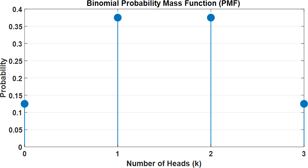
The PMF plot clearly visualises the probabilities for each possible number of heads. In this example, it shows that getting exactly 2 heads has a probability of 0.375, which we calculated earlier:

The CDF of a binomial distribution

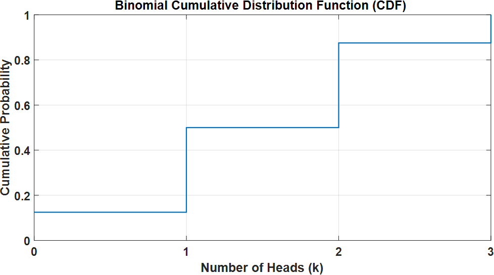
The CDF plot represents the cumulative probability of getting up to a certain number of heads. For instance, the CDF value at 2 heads tells us the probability of getting 0, 1, or 2 heads combined.

6. Properties of the Binomial Distribution

Let’s discuss some of the important properties of the BDF.

6.1. Identifying a Binomial Distribution

When we want to determine if a scenario follows a binomial distribution, we should check if it meets these conditions:

We have a fixed number of trials
Each trial results in two possible outcomes: success or failure
The probability of success is the same for each trial
The trials are independent of each other

If all these hold, we’re dealing with a binomial distribution.

6.2. Mean

The mean, or expected value, tells us the average number of expected successes. The formula is simple:

$[ \mu = n \cdot p ]$

This helps us figure out what to expect in the long run.

6.3. Variance

Variance shows us how spread out the results are. For a binomial distribution, it’s given by:

$[ \sigma^2 = n \cdot p \cdot (1 - p) ]$

It tells us how much the actual outcomes will differ from the average.

6.4. Standard Deviation

The standard deviation is just the square root of the variance:

$[ \sigma = \sqrt{n \cdot p \cdot (1 - p)} ]$

It gives a more intuitive sense of how far outcomes typically are from the mean.

6.5. Skewness

Skewness tells us if the distribution leans to one side. The formula is:

$[ \text{Skewness} = \frac{1 - 2p}{\sqrt{n \cdot p \cdot (1 - p)}} ]$

When p = 0.5 , the distribution is symmetric. If p < 0.5 , it’s skewed to the right, and if p > 0.5 , it’s skewed to the left.

6.6. Kurtosis

Kurtosis measures how "peaked" the distribution is. The formula is:

$[ \text{Kurtosis} = \frac{1 - 6p(1 - p)}{n \cdot p \cdot (1 - p)} ]$

A higher kurtosis means a sharper peak, while a lower one suggests a flatter shape.

7. Application

Let’s take a real-world scenario in the health sector: a vaccine trial. Suppose a vaccine is being tested and has an 80% success rate (i.e., it works for 80% of the patients). We run the trial on 15 patients and want to know how many will likely develop immunity.

7.1. Identifying a Binomial Distribution

This scenario meets the binomial distribution criteria:

Fixed number of trials: 15 patients are involved
Two possible outcomes: Each patient develops immunity (success) or does not (failure)
Probability of success : The probability that a patient develops immunity is 0.8
Independent trials: The response of each patient to the vaccine is independent of the others

7.2. Mean

The mean, or expected number of immune patients, is:

$[ \mu = n \cdot p = 15 \cdot 0.8 = 12 ]$

We expect 12 out of 15 patients to develop immunity.

7.3. Probability Calculations

Let’s break down the vaccine trial scenario using the binomial distribution formula step by step:

Number of trials patients
Success probability (vaccine works for 80% of patients)
Failure probability (vaccine fails for 20% of patients)
Number of successes = We can calculate the probability for different values of (e.g., 0 to 15)

Let’s calculate the probability of exactly 12 out of 15 patients developing immunity (i.e., k = 12 ):

$[ P(X = 12) = \binom{15}{12} (0.80)^{12} (0.20)^{3} ]$

First, calculate the binomial coefficient:

$[ \binom{15}{12} = \frac{15!}{12!(15-12)!} = \frac{15 \times 14 \times 13}{3 \times 2 \times 1} = 455 ]$

Now, calculate the powers:

$[ (0.80)^{12} \approx 0.0687 \quad \text{and} \quad (0.20)^{3} = 0.008 ]$

Finally, putting everything together:

$[ P(X = 12) = 455 \times 0.0687 \times 0.008 \approx 0.249 ]$

Thus, the probability of exactly 12 patients developing immunity is approximately 0.249, or 24.9%.

7.4. PMF and CDF Plots

Let’s now plot the PMF and CDF to visualize the distribution:

Histogram of the binomial distribution

The PMF plot shows how likely each number of immune patients is, with the highest probability around patients:

Example of Binomial CDF

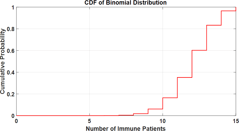
The CDF plot accumulates the probabilities, giving us a sense of how likely it is to have a certain number or fewer immune patients. For example, by looking at the CDF, we can easily estimate the probability of having fewer than 10 immune patients.

7.5. Variance

The variance, showing the spread of the number of immune patients:

$[ \sigma^2 = n \cdot p \cdot (1 - p) = 15 \cdot 0.8 \cdot (1 - 0.8) = 2.4 ]$

7.6. Standard Deviation

The standard deviation is:

$[ \sigma = \sqrt{2.4} \approx 1.55 ]$

Let’s illustrate this with a plot:

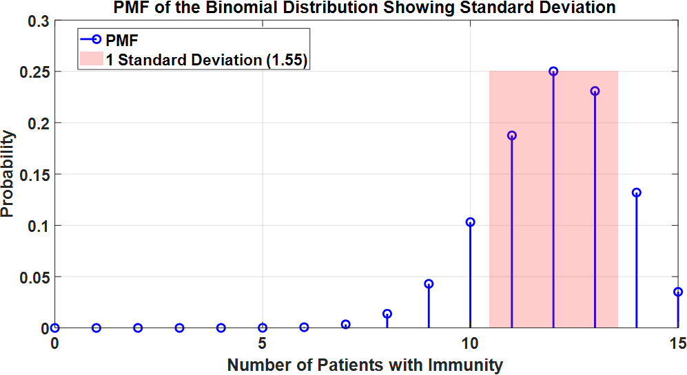
PMF with a highlighted region corresponding to the standard deviation around the mode

We fill the region on the plot from $\mu - \sigma$ to $\mu + \sigma$ with a red-filled area, showing one standard deviation 1.55 around the mean. This highlights that most immune patients will likely fall between ~10.45 and ~13.55, giving us a sense of the typical spread in the data.

7.7. Skewness

For our scenario:

$[ \text{Skewness} = \frac{1 - 2p}{\sqrt{n \cdot p \cdot (1 - p)}} = \frac{1 - 1.6}{\sqrt{15 \cdot 0.8 \cdot 0.2}} \approx -0.41 ]$

Since it’s negative, the distribution is slightly skewed to the left.

Let’s show the skewness of the distribution:

Left-skewed binomial distribution

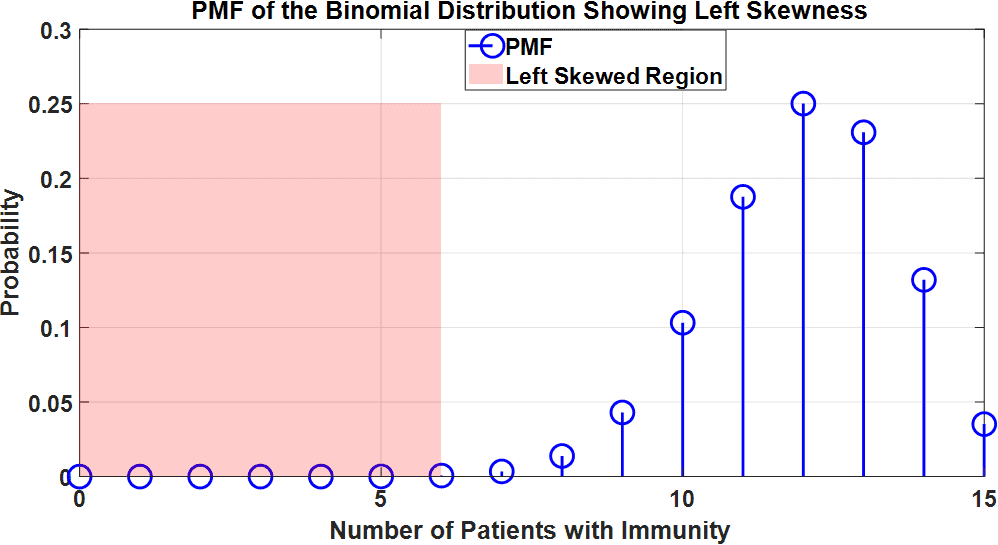
The left tail of the distribution is longer and thinner, which reflects the negative skewness value -0.41. This means that although the number of immune patients will mostly be close to the mean 12, there is a small chance of having fewer patients developing immunity.

7.8. Kurtosis

The kurtosis:

$[ \text{Kurtosis} = \frac{1 - 6p(1 - p)}{n \cdot p \cdot (1 - p)} \approx -0.3 ]$

This suggests a slightly flatter distribution than normal, as illustrated in the next plot:

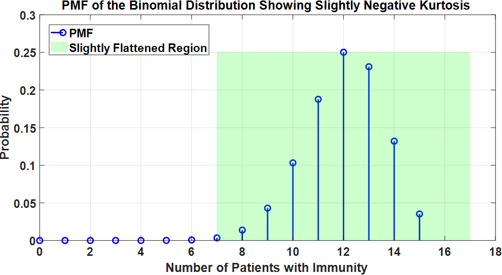
Platykurtic binomial distribution (negative excess kurtosis)

A slightly negative kurtosis -0.3 implies that the distribution is less sharply peaked (i.e., less concentrated around the mean) and has lighter tails, indicating fewer extreme outcomes. This visualization shows that the vaccine trial results are more likely to be spread out, with a flatter curve around the central values.

This simple scenario and its corresponding plots tie together all the properties of the binomial distribution and provide insight into how we can predict outcomes in a medical trial setting.

8. Conclusion

In this article, we have provided a solid background to understanding the binomial distribution and its properties and show how to quantify probabilities in scenarios with binary outcomes.

Persistence

REST

Security