模拟退火算法解释

1. Overview

In this tutorial, we’ll review the Simulated Annealing (SA), a metaheuristic algorithm commonly used for optimization problems with large search spaces. Additionally, we illustrate the SA optimization procedure and show how to minimize a function.

2. The Physics Behind the Algorithm

In general, SA is a metaheuristic optimization technique introduced by Kirkpatrick et al. in 1983 to solve the Travelling Salesman Problem (TSP).

The SA algorithm is based on the annealing process used in metallurgy, where a metal is heated to a high temperature quickly and then gradually cooled. At high temperatures, the atoms move fast. Moreover, when the temperature is reduced, their kinetic energy decreases as well. At the end of the annealing process, the atoms fall into a more ordered state. Additionally, the material becomes more ductile and easier to work with.

Similarly, in SA, a search process starts with a high-energy state (an initial solution) and gradually lowers the temperature (a control parameter) until it reaches a state of minimum energy (the optimal solution).

We can apply SA in a wide range of optimization problems, such as TSP, protein folding, graph partitioning, and job-shop scheduling. In particular, the main advantage of SA is its ability to escape from local minima and converge to a global minimum. Moreover, SA is relatively easy to implement and doesn’t require prior knowledge of the search space.

3. Algorithm

At first, the simulated annealing process starts with an initial solution. Furthermore, SA iteratively improves the current solution by randomly perturbing it and accepting the perturbation with a certain probability.

The probability of accepting a worse solution is initially high. However, as the number of iterations increases, the probability of accepting a worse solution gradually decreases. Therefore, the accuracy of the solution depends on the number of iterations SA performs.

The SA algorithm is quite simple, and we implement it straightforwardly, as described below.

3.1. Define the Problem

First, we need to define the problem to optimize. It involves defining the energy function, i.e., the function to minimize or maximize. For example, if we want to minimize a real-valued function of two variables, e.g., , the energy corresponds to the function itself. In the case of the TSP, the energy related to a sequence of cities is represented by the total length of the travel.

Once we define the energy function, we need to set the initial temperature value and the initial candidate solution. Moreover, we can set the initial temperature value and the initial candidate solution either randomly or using some heuristic method. Furthermore, the next step is to compute the energy of the initial candidate solution.

3.2. Define the Perturbation Function

Next, we define a perturbation function to generate new candidate solutions. Thus, this function should generate solutions that are close to the current solution but not too similar. For example, if we want to minimize a function , we can randomly perturb the current solution by adding a random value between -0.1 and 0.1 to both and . In the case of the TSP, we can generate a new candidate solution by swapping two cities in the travelling order of the current solution.

3.3. Acceptance Criterion

The acceptance criterion determines whether a new solution is accepted or rejected. Moreover, the acceptance depends on the energy difference between the new solution and the current solution, as well as the current temperature.

The classic acceptance criterion of SA comes from statistical mechanics, and it is based on the Boltzmann probability distribution. A system in thermal equilibrium at temperature can be found in a state with energy with a probability proportional to

(1)  

where is the Boltzmann constant. Hence, at low temperatures, there is a small chance that the system is in a high-energy state. It plays a crucial role in SA because an increase in energy allows escape from local minima and finds the global minimum.

Based on the Boltzmann distribution, the following algorithm defines the criterion for accepting an energy variation at temperature :

algorithm AcceptanceFunction(T, ΔE):
    // INPUT
        T = the temperature
        ΔE = the energy variation between the new candidate solution and the current one
    // OUTPUT
        Returns true if the new solution is accepted. Otherwise, returns false.

    if ΔE < 0:
        return true
    else:
        r <- generate a random value in the range [0, 1)
        if r < exp(-ΔE / T):
            return true
        else:
            return false

Thus, a candidate solution with lower energy is always accepted. Conversely, a candidate solution with higher energy is accepted randomly with probability (for our purpose, we can set ). Moreover, we can implement the latter cases by comparing the probability with a random value generated in the range ![0, 1).

3.4. Temperature Schedule

The temperature schedule determines how the temperature of the system changes over time. In the beginning, the temperature is high so that the algorithm can explore a wide range of solutions, even if they are worse than the current solution. As the iterations increase, the temperature gradually decreases. Hence, the algorithm becomes more selective and accepts better solutions with higher probability.

Here, we can obtain a simple scheduling method by multiplying the current temperature by a factor , where :

   

Hence, it ensures the temperature decreases gradually over time as the value of is always less than 1.

3.5. Run the SA Algorithm

Finally, we run the algorithm iteratively by applying the perturbation function and acceptance criterion to the current solution. Moreover, the algorithm terminates when the temperature has cooled to a certain level or when the energy of the current solution is lower than a fixed threshold .

Here’s the pseudocode of SA:

algorithm SimulatedAnnealingOptimizer(T_max, T_min, E_th, α):
    // INPUT
        T_max = the maximum temperature
        T_min = the minimum temperature for stopping the algorithm
        E_th = the energy threshold to stop the algorithm
        alpha = the cooling factor
    // OUTPUT
        The best found solution

    T <- T_max
    x <- generate the initial candidate solution
    E <- E(x)  // compute the energy of the initial solution

    while T > T_min and E > E_th:
        x_new <- generate a new candidate solution
        E_new <- compute the energy of the new candidate x_new
        ΔE <- E_new - E

        if Accept(ΔE, T):
            x <- x_new
            E <- E_new

        T <- T * alpha  // cool the temperature

    return x

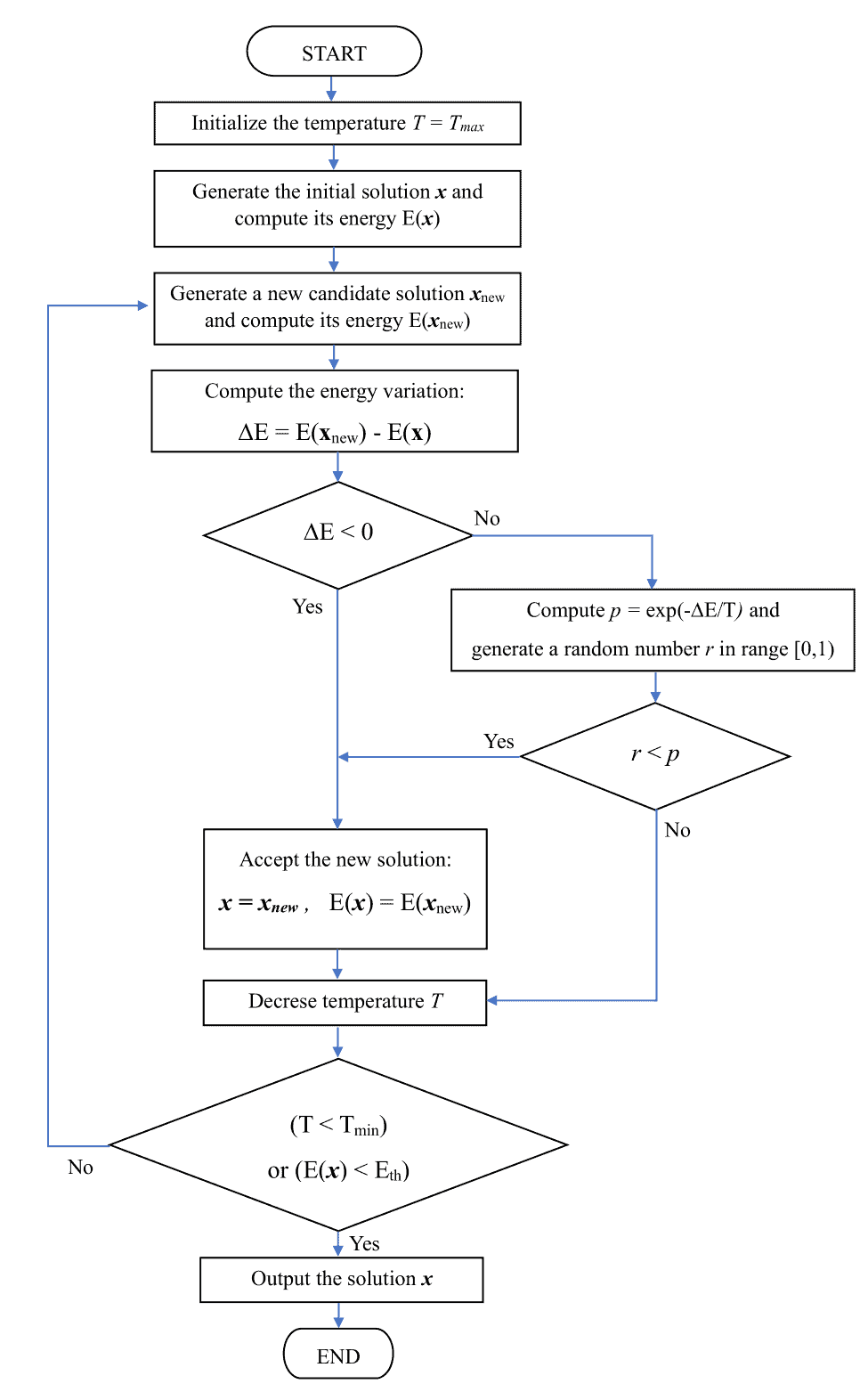
4. SA Flowchart

Here, we provide a detailed flowchart representing all steps of SA:

5. Example

To better understand the algorithm, we use SA to illustrate the minimization of the function . First, we used as search space a grid of size 101 101 placed in the square area defined by . Furthermore, we set the cooling rate and the initial solution . Additionally, at each step, we generate a new solution by randomly shifting the current solution by in and direction.

Here’s an animation showing the candidate solution, its energy, and the temperature at each step:

Thus, we can observe that SA accepts the worse solutions when the temperature is high. Conversely, when the temperature is low (e.g., ), the algorithm is more selective, and better solutions are accepted with higher probability.

6. Conclusion

In this article, we provided an overview of the SA algorithm. Furthermore, we illustrated the optimization procedure and provided a practical example of its application.