1. Introduction
In this article, we’ll introduce the fundamental concepts behind Treaps and examine how they combine binary search and heap behavior.
Unlike other tree data structures, Treaps prevent devolving into straight lines in the event that the values inserted were already in sorted order. We’ll demonstrate how Treaps benefit from the expected height of a random BST, achieving logarithmic expected time for insertion, deletion, and search operations.
2. Treaps
To understand Treaps, let’s start by recalling two of the most fundamental data structures in Computer Science: the tree and the heap. A Treap is a deliberate portmanteau of tree and heap, intended to highlight the properties of these two data structures.**
On the one hand, a Treap enforces the Binary Search Tree (BST) property on node values. That is, for any node, all values in its left subtree are smaller, and all values in its right subtree are greater. This guarantees that lookups, insertions, and deletions proceed just as they would in an ordinary BST.
On the other hand, a Treap has a heap property on node priorities. In a min-heap Treap, each node’s priority is no greater than the priorities of its children; in a max-heap Treap, each node’s priority is no smaller than the priorities of its children.
Because these two constraints must hold, the shape of the tree reflects both the ordering of the keys and the ordering of the priorities. As a result, assigning random priorities simulates the expected structure of a random BST. Similarly, whenever the heap property is violated, the tree performs rotations to restore heap order without breaking the BST property.
Let’s consider an example of a Treap:
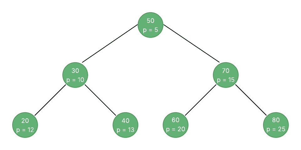
The diagram above shows a fully populated tree whose nodes store a key (for BST ordering) and a random priority (for heap ordering). This tree illustrates how every parent’s key follows the BST rules while its priority maintains the min-heap property.
3. Insertion
When inserting a key into the Treap, we first generate a random priority for the new element and check whether the key already exists to avoid duplicates. If the key is not present, we wrap it in a new node containing both its value and priority, then invoke the InsertNode() function helper to place it in the correct position and restore heap order as needed:
function Insert(treap, key):
    // INPUT
    //     treap = the Treap data structure
    //     key   = the key to insert
    // OUTPUT
    //     Inserts a new node with 'key' into 'treap', maintaining BST and heap properties

    priority <- rng.next()                      // generate a random priority
    if Search(treap, key) = true:              // avoid duplicates
        return
    node    <- new Node(key, priority)         // create the new node
    treap.root <- InsertNode(treap.root, node)  // insert into the tree
end function
The InsertNode() function handles the balancing logic. It recursively descends as in a standard BST. That is, if the new node’s key is smaller than the current root’s key, it goes into the left subtree. Yet, if greater, into the right. After linking in the new node (or identifying a duplicate), we compare the child’s priority against the parent’s.
Whenever a child’s priority violates the heap condition, being smaller than its parent’s for min-heap, we perform a rotation (either left or right) to lift that child upward while preserving the BST order. The function then returns the subtree root back up the recursion:
function InsertNode(root, node):
    // INPUT
    //     root = current subtree root
    //     node = node to insert (with key + priority)
    // OUTPUT
    //     Returns the new subtree root after insertion and any necessary rotations

    if root = null:
        return node

    if node.key < root.key:
        root.left <- InsertNode(root.left, node)
        if root.left.priority < root.priority:  // heap check
            root <- RotateRight(root)            // restore heap property
    else if node.key > root.key:
        root.right <- InsertNode(root.right, node)
        if root.right.priority < root.priority: // heap check
            root <- RotateLeft(root)             // restore heap property
    // else key == root.key: do nothing

    return root
end function
4. Deletion
Removing a key from a Treap combines BST lookup with heap-based rotations to maintain both properties. We begin by calling the public Delete() function on the root; it simply delegates to DeleteNode(), which performs the recursive removal and uses rotations to “push down” the node to be deleted until it becomes a leaf. At that point, it can be removed without violating either property:
function Delete(treap, key):
    // INPUT
    //     treap = the Treap data structure
    //     key   = the key to delete
    // OUTPUT
    //     Removes the node with 'key' from 'treap', preserving BST and heap properties

    treap.root <- DeleteNode(treap.root, key)
end function
The DeleteNode() helper searches for the node as in an ordinary BST. If the key is smaller or larger than the current root’s key, it recurses left or right. Once it finds the target node, there are three cases: if it has no children, we simply drop it by returning null. if it has one child, we return that child directly. Finally, if it has two children, we compare the priorities of the left and right child and rotate the root in the direction that brings the higher-priority child to the top.
This rotation pushes the deleted node down one level, and we recurse again until it becomes a leaf:
function DeleteNode(root, key):
    // INPUT
    //     root = current subtree root
    //     key  = key to delete
    // OUTPUT
    //     Returns the new subtree root after deletion and any necessary rotations

    if root = null:
        return null

    if key < root.key:
        root.left  <- DeleteNode(root.left, key)
    else if key > root.key:
        root.right <- DeleteNode(root.right, key)
    else
        // found the node to delete
        if root.left = null and root.right = null:
            return null
        else if root.left = null or (root.right != null and root.right.priority < root.left.priority):
            root <- RotateLeft(root)
            root.left <- DeleteNode(root.left, key)
        else
            root <- RotateRight(root)
            root.right <- DeleteNode(root.right, key)
    return root
end function
By repeatedly rotating the target node downward according to heap order, we guarantee that it eventually reaches a position with at most one child. At that point, a simple pointer replacement safely removes it without breaking the BST or heap characteristics, all in the expected O(log n) time.
5. Search
Searching for a key in a Treap is exactly the same as in a standard binary search tree: we ignore priorities entirely and traverse left or right based on comparisons until we either find the key or reach a null subtree. This guarantees an expected O(log n) search time since the Treap’s random priorities keep its height-balanced:
function Search(treap, key):
    // INPUT
    //     treap = the Treap data structure
    //     key   = the key to search for
    // OUTPUT
    //     Returns true if 'key' exists in 'treap', false otherwise

    return SearchNode(treap.root, key)
end function

function SearchNode(node, key):
    // INPUT
    //     node = current subtree root
    //     key  = the key to search for
    // OUTPUT
    //     Returns true if 'key' is found in this subtree

    if node = null:
        return false

    if key < node.key:
        return SearchNode(node.left, key)
    else if key > node.key:
        return SearchNode(node.right, key)
    else
        return true   // key == node.key
end function
In this implementation, we start at the Treap’s root and compare the target key to the current node’s key. If the target is smaller, we recurse into the left subtree; if larger, into the right. When we reach a node whose key matches, we return true. If we hit a null pointer, the key is not present, and we return false. Because the Treap remains balanced in expectation, this simple BST search runs on average in O(log n) time.
6. Key Differences Between Treaps and Other Tree Data Structures
Let’s compare Treaps with other tree-like data structures, focusing on their most common operations and structure:
Balancing Principle
Avg. Search / Insert / Delete
Worst-Case Search
Worst-Case Insert
Worst-Case Delete
Typical Use Cases
Treap
Randomized heap priority + BST order
O(log n)
O(n)
O(n)
O(n)
Near-balanced maps/sets, persistent structures
BST
None
O(log n)
O(n)
O(n)
O(n)
Small/simple dictionaries
AVL Tree
Height strictly balanced
O(log n)
O(log n)
O(log n)
O(log n)
Predictable read/write indexes, embedded DBs
Trie
None
O(n)
O(n)
O(n)
O(n)
Autocomplete, routing tables, prefix lookups
7. Conclusion
In this article, we explored Treaps – a randomized data structure that combines BST ordering with heap priorities. We introduced the core concepts behind Treaps, and walked through pseudocode for insertion, deletion, and search.
By assigning random priorities and performing rotations whenever the min-heap invariant is violated, Treaps maintain the expected logarithmic height. As a result, all core operations (insert, delete, and search run) in O(log n) time on average, work as an alternative to strictly balanced trees.