Understand Bootstrapping in Statistical Analysis

1. Introduction

In this tutorial, we’ll focus on bias estimation and confidence intervals via bootstrapping in one-sample settings. We’ll explain how and why bootstrap works and show how to implement the percentile and reversed bootstrapped confidence intervals in Python.

2. When Is Bootstrap Useful?

Let’s say we want to estimate the efficiency of an algorithm. So, we define 50 various inputs, execute our algorithm, and record the execution times. To make the average estimate more robust to outliers (which represent too easy and too hard inputs), we drop the bottom 10% and top 10% values and compute the mean of the inner 80%. This is an example of a trimmed mean.

To find the confidence interval around the computed value or to make other statistical inferences, we need to know the distribution of the trimmed mean as a statistic (a random variable). By the central limit theorem, the mean of a sample is asymptotically normally distributed, but that’s not necessarily the case with the mean of a trimmed sample.

The bootstrap technique is useful when we don’t know the distribution of a sample statistic because analytical derivation is too complex or impossible. Bootstrap allows us to approximate the distribution and use it for statistical inference.

3. Bootstrap

If we could draw sufficiently many samples from the underlying population and calculate a statistic $\boldsymbol{t}$ for each sample, we could approximate the statistic’s sampling distribution:

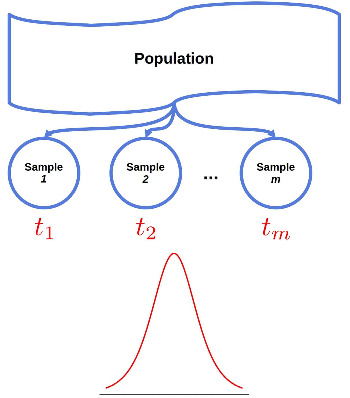
Let’s say we repeated the run-time experiment 1000 times. In replication, we ran the algorithm 50 times and computed the trimmed mean. That way, we would get an empirical approximation of the trimmed mean’s distribution.

However, resampling from the population may be hard or impossible. For instance, the algorithm may be expensive to execute because it requires extensive computational resources.

3.1. The Bootstrap Idea

In bootstrapping, we define an approximate mathematical model (i.e., distribution) from which we can sample straightforwardly. So, instead of resampling from the true population (a distribution with CDF ), we draw a large number of resamples (called bootstrap samples) from an approximation $F^* \approx F$ :

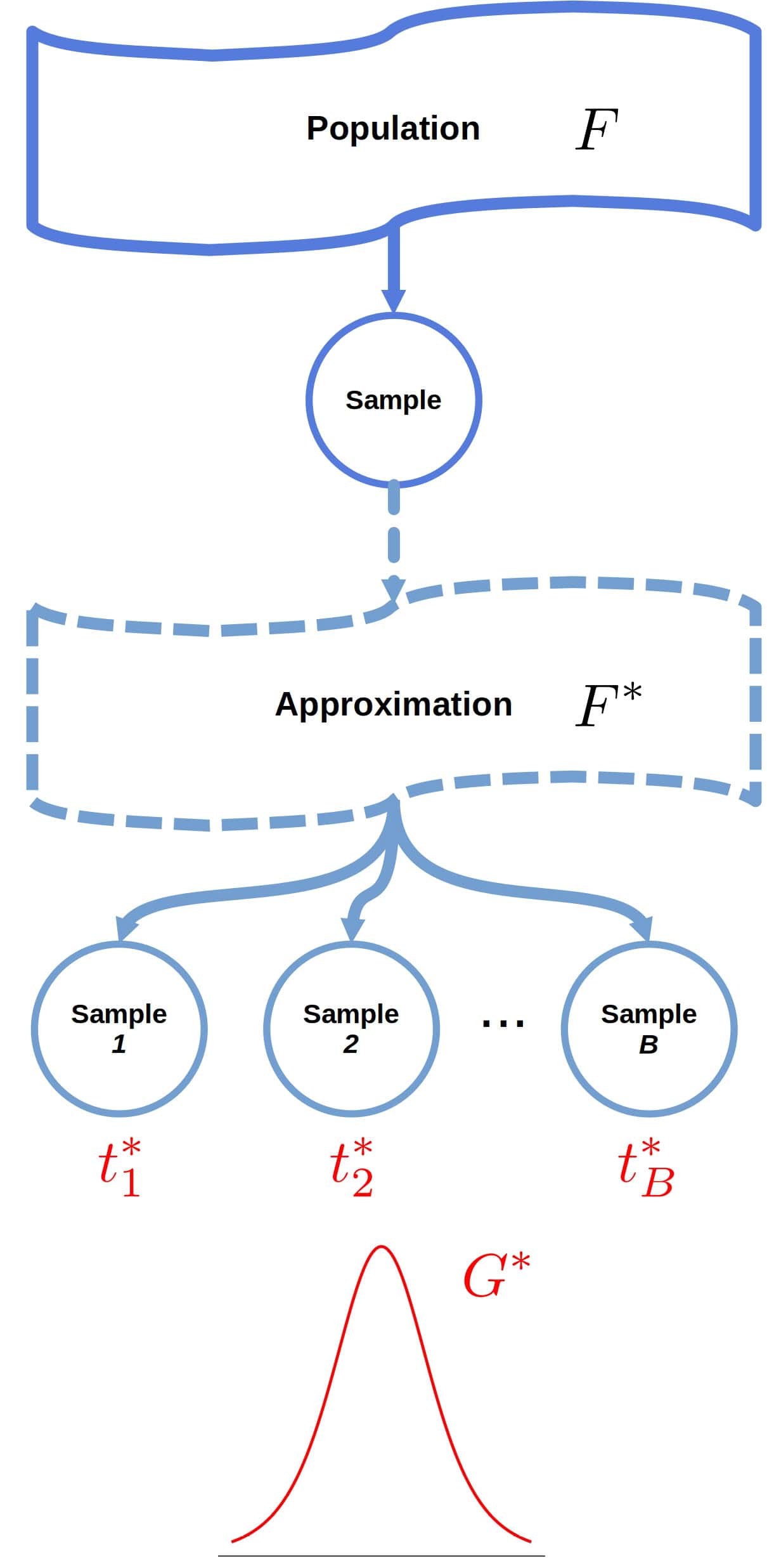
This way, we compute G^* , the CDF of the statistic T^*=t(X^*) , where $X^* \sim F^*$ . Under certain conditions, one of which is that the approximation F^* is good enough, we can expect G^* to have the same shape and spread as , the CDF of T=t(X) when $X \sim F$ (we would get if we could resample from at will).

Note that if we can derive the distribution G^* analytically, we don’t need bootstrap samples. However, that’s not the case for most statistics. In practice, we set to a high enough value and approximate G^* by sampling.

3.2. Types of Bootstrap

We can categorize bootstrap techniques depending on how they obtain F^* .

Parametric bootstrap assumes the family $\boldsymbol{\Phi}$ of $\boldsymbol{F}$ , estimates its parameters from the initial sample $\boldsymbol{x_1, x_2, \ldots, x_n}$ , and defines $\boldsymbol{F^*}$ as the CDF in family $\boldsymbol{\Phi}$ with those parameters. For example, we can assume that is the CDF of an exponential distribution (with the density $f(x)=\lambda e^{-\lambda x}$ ), and use $x_1, x_2, \ldots, x_n$ to find an estimate $\lambda^*$ of $\lambda$ . Then, F^* will have the density $f^*(x)=\lambda^* e^{-\lambda^* x}$ .

Smoothed bootstrap uses kernel density estimation to arrive at $\boldsymbol{F^*}$ .

Nonparametric bootstrap assumes nothing about the shape or family of $\boldsymbol{F}$ and uses the empirical CDF based on $\boldsymbol{x_1, x_2, \ldots, x_n}$ as \boldsymbol{F^*}. Here, we draw from F^* by sampling from $x_1, x_2, \ldots, x_n$ with replacement.

4. Bootstrap and Statistical Inference

4.1. Bootstrap Approximates the Error Distribution

Although we expect their shapes and spread to be similar, the means of G^* and need not be identical. The bootstrapped t^* values will fluctuate around the mean of G^* . Let’s denote it as t(F^*)+b^* , where b^* is the potential bias, and t(F^*) is the population value of interest with respect to F^* . This mean isn’t necessarily equal to the mean of ( =t(F)+b ), where t(F) is the value of in the actual population.

Therefore, another condition for the similarity of shapes (and spread) is that they don’t depend on the locations, i.e., that the moments of don’t depend on the mean of and that the moments of G^* don’t depend on the mean of G^* .

However, all said and done, even if the shapes are similar, the locations can and usually differ.

Then, why is G^* useful? The approximation F^* should be such that we can easily compute t(F^*) . Subtracting t(F^*) from a G^* -distributed random variable, we get a model for the error of t(X^*) :

$[Err^* = T^* - t(F^*) \qquad T^* \sim G^*]$

Because the shapes are the same (or similar enough), the error of t(X) follows a similar distribution:

$[Err^* \approx Err = T - t(F) \qquad T \sim G]$

We can use the distribution of Err to analyze the bias of and construct the confidence intervals for t(F) .

Let $x_1, x_2, \ldots, x_n$ be the original sample (from ) and let $t(x_1, x_2, \ldots, x_n)$ be the original estimate of t(F) .

In non-parametric bootstrap, $\boldsymbol{F^*}$ is the ECDF $\boldsymbol{\widehat{F}}$ based on the original sample $\boldsymbol{x_1, x_2, \ldots, x_n}$ , so $\boldsymbol{t(F^*)=t(\widehat{F})=t(x_1, x_2, \ldots, x_n)}$ .

4.2. Bias

The value E(Err^*) estimates the bias with respect to F^* .

Under the assumption that if $F^* \approx F$ , we’ll have $b^*\approx b$ , so we can use E(Err^*) as the bias estimate for in the original population.

If it’s non-zero, we can consider a biased statistic. Otherwise, we say it’s unbiased or a consistent estimator.

We may be tempted to use the bias estimate to correct $t(x_1, x_2, \ldots, x_n)$ , but such corrections may do more harm than good because bias estimates can be unstable.

4.3. Reversed Confidence Intervals

Let’s say the statistic is unbiased. Let the $\alpha/2$ and $(1-\alpha/2)$ quantiles of Err be $q_{\alpha}$ and $q_{1-\alpha/2}$ . In practice, we sort the $\boldsymbol{t^*}$ values and use those at positions $\boldsymbol{[\alpha B /2]}$ and $\boldsymbol{[(1-\alpha/2) B]}$ . Then:

$[\begin{aligned} P\left( T - t(F) \leq q_{\alpha/2} \right) &\approx \alpha/2 \\ P\left( T - t(F) \geq q_{1-\alpha/2} \right) &\approx \alpha/2 \end{aligned}]$

From there, we get:

$[P\left( T - q_{1-\alpha/2} < t(F) < T - q_{\alpha/2}\right) \approx 1 - \alpha]$

So, the interval for t(F) is:

$[\left(t(x_1, x_2, \ldots, x_n) - q_{1-\alpha/2}, t(x_1, x_2, \ldots, x_n) - q_{\alpha/2}\right)]$

Since the quantiles are reversed in the final interval, we call these bootstrap intervals reversed.

4.4. Percentile Confidence Intervals

There are other bootstrap intervals. We’ll cover the construction of percentile confidence intervals.

The percentile method has an even stronger assumption that $\boldsymbol{G^* \approx G}$ in shape, spread, and location. So, in this method, we treat the quantiles $\boldsymbol{q_{\alpha}}$ and $\boldsymbol{q_{1-\alpha/2}}$ of $\boldsymbol{G^*}$ as the corresponding quantiles of $\boldsymbol{G}$ .

Therefore, the percentile interval (for t(F) ) is:

$[(q_{\alpha/2}, q_{1-\alpha/2})]$

Reversed and percentile intervals are easy to compute but fail if their assumptions aren’t met.

4.5. Bootstrap Assumptions

Bootstrap assumes that the bootstrapped distribution G^* is similar enough to the actual distribution of the statistic of interest.

For that reasoning to hold, $\boldsymbol{F^*}$ must approximate $\boldsymbol{F}$ well, and $\boldsymbol{t}$ should be robust to small changes in its argument.

The former condition is there because we can’t use F^* as a proxy for if it isn’t precise. The latter condition ensures that small deviations of F^* from don’t translate to large deviations of G^* from (this property is known as smoothness). If these conditions aren’t met, bootstrap won’t be useful.

There may be additional assumptions depending on the bootstrap technique. For example, the confidence-interval methods we discussed assume that the shape and spread of G^* and don’t depend on their location parameters.

5. Python Implementation

Let’s implement reversed and percentile interval methods in Python.

We’ll use nonparametric bootstrap, which means we’ll take bootstrap samples from the original sample with replacement.

We’ll need numpy and scipy:

import numpy
import scipy.stats

5.1. Code for Reversed Intervals

Here’s the code for reversed intervals:

def bootstrap_reversed_ci(x, alpha, B):
    # Compute the sample statistic
    t = scipy.stats.trim_mean(x, 0.1)

    # Draw bootstrap samples
    n = len(x)
    x_bootstrap = np.random.choice(x, size=(B, n), replace=True)

    # Compute the bootstrap statistics
    t_bootstrap = scipy.stats.trim_mean(x_bootstrap, 0.1, axis=1)

    # Find the error distribution
    # (In non-parametric bootstrap, the population mean of t_bootstrap is t.)
    err_bootstrap = t_bootstrap - t

    # Find the quantiles
    q_lower, q_upper = np.quantile(err_bootstrap, (alpha/2, 1 - alpha/2))
    
    return t, (t - q_upper, t - q_lower)

Here, x_bootstrap is a $B \times n$ matrix. By specifying axis=1 in scipy.stats.trim_mean(), we calculate the trimmed mean for each row and obtain a $B \times 1$ numpy array. This and other calculations are vectorized to improve performance.

The array err_bootstrap holds the differences t_i^* - t(F^*) for $i=1,2,\ldots, B$ . Since we use the nonparametric bootstrap, t(F^*) is the trimmed mean of the original sample x.

Finally, we use the alpha/2 and (1-alpha/2) quantiles of err_bootstrap to define the confidence interval and return it alongside the sample trimmed mean.

5.2. Code for Percentile Intervals

Here’s the code for percentile intervals:

def bootstrap_percentile_ci(x, alpha, B):
    # Compute the sample statistic
    t = scipy.stats.trim_mean(x, 0.1)
    
    # Draw bootstrap samples
    n = len(x)
    x_bootstrap = np.random.choice(x, size=(B, n), replace=True)

    # Compute the bootstrap statistics
    t_bootstrap = scipy.stats.trim_mean(x_bootstrap, 0.1, axis=1)

    # Find the quantiles
    q_lower, q_upper = np.quantile(t_bootstrap, (alpha/2, 1 - alpha/2))
    
    return t, (q_lower, q_upper)

Here, we also perform vectorized calculations. The main difference is that we don’t compute the error distribution. Instead, we use the alpha/2 and (1 – alpha/2) quantiles of the array t_bootstrap of the bootstrapped statistics as the lower and upper boundaries of the confidence interval.

5.3. Results

Let’s see how to use these functions. As an example, we draw the original sample from an exponential distribution $\lambda=1/2$ , but any other distribution is suitable. We draw B=1000 bootstrap samples and aim for the coverage of $1-\alpha=1-0.05=0.95$ :

x = scipy.stats.expon.rvs(scale=2, size=50)
print(bootstrap_reversed_ci(x, 0.05, 1000))
print(bootstrap_percentile_ci(x, 0.05, 1000))

Here’s an example output:

1.685 (1.237, 2.0355)
1.685 (1.2081, 2.0595)

We see the sample trimmed mean and the reversed and percentile intervals. Both methods produced similar results and captured the true trimmed mean of approximately 1.6615.

To use these bootstrap functions with another statistic, we need to replace scipy.stats.trim_mean.

6. Conclusion

In this article, we explained the ideas behind bootstrap in statistics and showed how to estimate the bias and compute confidence intervals.

Bootstrap is useful when we don’t know the sampling distribution of a statistic, but it can fail if its assumptions aren’t met.

Persistence

REST

Security