How Does Kernel Density Estimation Work?

1. Introduction

In this tutorial, we’ll explore kernel density estimation (KDE), a method for estimating the probability density function of a continuous variable. KDE is valuable in statistics and data science because it provides a smooth distribution estimate, which is useful when we know little about the distribution it follows and have no grounds to make assumptions about its family or other properties.

We’ll cover the basics of KDE, including a simple example, the math behind it, and guidelines for choosing a suitable kernel and bandwidth. Additionally, we’ll implement KDE in Python and review how to estimate the bandwidth for optimal results.

We’ll focus on the kernel density estimation KDE for univariate data. The rules and principles are similar for the multivariate KDE, but the math is different.

2. What Is Kernel Density Estimation?

Kernel Density Estimation (KDE) is a method for approximating a random variable’s probability density function (PDF) using a finite sample.

KDE doesn’t assume a specific data distribution (like normal or exponential); instead, it estimates the distribution’s shape directly from the data points.

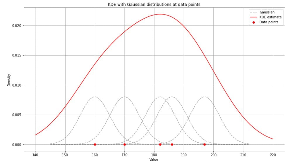
We can consider KDE a way of “smoothing out” each data point by centering a small distribution on each data point. These local distributions, kernels, are then combined to create a continuous curve representing the estimated density (of the global distribution):

Kernel density estimation with Gaussian distributions

KDE is beneficial when we lack information about the underlying distribution of data.

It offers a more flexible approach than histograms by creating a smooth distribution curve instead of discrete bins. KDE is widely used in exploratory data analysis to detect patterns and identify outliers.

3. How Does Kernel Density Estimation Work?

Suppose we have a small dataset with the heights (in cm) of a group of people:

160, 170, 182, 186, 197

KDE takes each height value, centers a kernel function (often a Gaussian curve) at each data point, and then averages these curves to form a smooth density estimate.

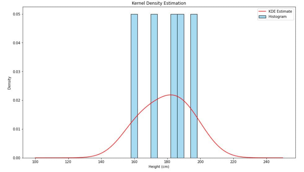
Here’s an example of a KDE overlaid on a histogram of these heights:

Kernel density estimation example

Mathematically, we estimate the density at any point as follows:

(1) $\begin{equation*} \hat{f}(x) = \frac{1}{n \cdot h} \sum_{i=1}^{n} K\left(\frac{x - x_i}{h}\right), \end{equation*}$

where:

is the number of data points
$x_{i}$ ( $i=1,2, \ldots,n$ ) are data points
is the bandwidth that controls the smoothness of the estimate
and is the kernel function (usually a Gaussian function)

The kernel function shapes the individual data points into small distributions, and the bandwidth determines the spread of each kernel.

3.1. How to Select a Kernel for KDE?

The most commonly used kernel is the Gaussian function:

(2) $\begin{equation*} K(u) = \frac{1}{\sqrt{2\pi}} e^{-\frac{u^2}{2}}. \end{equation*}$

However, there are others, such as Epanechnikov, uniform, and triangular:

$[ \begin{aligned} \text{Epanechnikov}(u) &= \frac{3}{4} (1 - u^2), & \text{for } |u| \leq 1 \text{ and } 0 \text{ otherwise} \\ \text{Uniform}(u) &= \frac{1}{2}, & \text{for } |u| \leq 1 \text{ and } 0 \text{ otherwise} \\ \text{Triangular}(u) &= (1 - |u|), & \text{for } |u| \leq 1 \text{ and } 0 \text{ otherwise} \\ \end{aligned} ]$

Still, the Gaussian kernel is preferred because it produces smooth, continuous curves and performs well with most data.

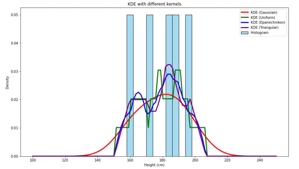
kernel density estimation with different kernels

As we can see, the red line representing the KDE estimator using the Gaussian kernel is smoother and fits the data more naturally.

3.2. Numerical Example

Let’s say we want to calculate the KDE for height x = 180 with bandwidth h = 10 and a Gaussian kernel . We’ll use the same dataset of heights (160, 170, 182, 186, 197) as before.

Then, our estimate of density at x=180 is:

$[ \begin{aligned} \hat{f}(180) &= \frac{1}{n \cdot h} \sum_{i=1}^{n} K\left(\frac{180 - x_i}{h}\right) \\ &= \frac{1}{5 \cdot 10} \sum_{i=1}^{5} \frac{1}{\sqrt{2\pi}} e^{-\frac{\left(\frac{180 - x_i}{10}\right)^2}{2}} \\ &= \frac{1}{50\sqrt{2\pi}} \sum_{i=1}^{5} e^{-\frac{(180 - x_i)^2}{200}} = \\ &= \frac{1}{50\sqrt{2\pi}} (e^{-\frac{(180 - 160)^2}{200}} + e^{-\frac{(180 - 170)^2}{200}} + e^{-\frac{(180 - 182)^2}{200}} + e^{-\frac{(180 - 186)^2}{200}} + e^{-\frac{(180 - 197)^2}{200}}) \\ &\approx 0.008 \cdot (0.14 + 0.61 + 0.98 + 0.84 + 0.24) \approx 0.0225 \end{aligned} ]$

4. How to Select a Bandwidth for KDE?

Bandwidth plays a crucial role in the KDE output.

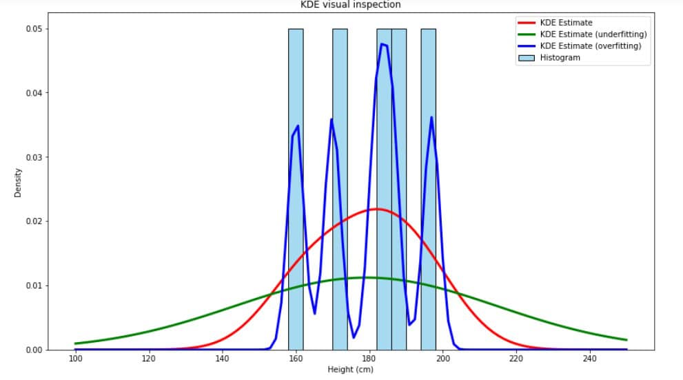
A small $\boldsymbol{h}$ can result in an estimate that’s too “spiky” (overfitting), while a large $\boldsymbol{h}$ may oversmooth the data, hiding essential details (underfitting).

There are several methods for selecting bandwidth:

Silverman’s rule of thumb
Cross-validation
Visual inspection
Sheather-Jones method (plug-in method)

Each method has different strengths, depending on the dataset and the precision required.

4.1. Silverman’s Rule of Thumb

Silverman’s rule of thumb is a widely used, straightforward method for bandwidth selection. It assumes the data is approximately normally distributed and calculates the bandwidth using the formula:

(3) $\begin{equation*} h = 1.06 \sigma n^{-1/5}, \end{equation*}$

where $\sigma$ is the standard deviation of the data, and is the number of data points. Silverman’s method is quick and easy to compute but may be suboptimal for data with complex or non-normal distributions.

4.2. Cross-Validation

Cross-validation, especially leave-one-out cross-validation (LOOCV), is a data-driven approach to finding an optimal bandwidth by minimizing the error in the density estimate.

It works by excluding one data point at a time, estimating the density based on the remaining points, and then measuring the error.

The objective is to find the bandwidth that minimizes the mean integrated squared error (MISE):

(4) $\begin{equation*} \text{MISE}(h) = \int \left( f(x) - \hat{f}_h(x) \right)^2 \, dx. \end{equation*}$

Practically, LOOCV uses the data to approximate this by summing over all observations:

(5) $\begin{equation*} h_{\text{opt}} = \arg \min_h \sum_{i=1}^{n} \left( f(x_i) - \hat{f}_h(x_i) \right)^2, \end{equation*}$

where $\hat{f}_h(x_{i})$ is the leave-one-out estimated density at point $x_{i}$ , computed by excluding $x_{i}$ from the KDE $f(x_{i})$ .

This method is computationally intensive but yields an empirically optimal bandwidth, which is particularly useful for non-normal and complex data distributions.

4.3. Sheather-Jones Method

The Sheather-Jones method, also known as a plug-in method, is an advanced option that calculates bandwidth by directly estimating an optimal that minimizes an approximation of the MISE.

This approach often produces better results than Silverman’s rule, especially when precision is needed. However, Silverman’s rule is a quick and easy solution, ideal for simple distributions.

4.4. Visual Inspection

Visual inspection is a more informal and practical way to select bandwidth.

We can quickly assess which bandwidth best captures the distribution by generating KDE plots with several bandwidth values and visually inspecting the fit.

This method is suitable for exploratory analysis and small datasets where quick, rough tuning of suffices. In the example below, visual inspection reveals that the red distribution makes more sense than green (underfitting) or blue (overfitting):

Kernel density example with overfitting and underfitting

5. Kernel Density Estimation in Python

As a simple example, we’ll implement a KDE for our small dataset of heights. We’ll determine the bandwidth using Silverman’s rule of thumb. The estimated density will be presented as a plot together with the data histogram:

import numpy as np
import seaborn as sns
from scipy.stats import gaussian_kde
import matplotlib.pyplot as plt

# sample data
data = np.array([160, 170, 182, 186, 197])

# calculate the optimal bandwidth using Silverman's rule
std_dev = np.std(data)
n = len(data)
bandwidth = 1.06 * std_dev * n ** (-1/5)

# perform KDE with gaussian_kde
kde = gaussian_kde(data, bw_method=bandwidth / std_dev)

# plotting
x_values = np.linspace(100, 250, 100)  # Range for plot
plt.figure(figsize=(8, 6))

bin_width = 4
bins = np.arange(min(data) - bin_width / 2, max(data) + bin_width, bin_width)
sns.histplot(data, bins=bins, kde=False, color="skyblue", label="Histogram", stat="density")
plt.plot(x_values, kde(x_values), color="red", label="KDE Estimate")
plt.legend()
plt.xlabel("Height (cm)")
plt.ylabel("Density")
plt.title("Kernel Density Estimation")
plt.show()

The generated plot looks like this:

Kernel density estimation example

The KDE was estimated using Silverman’s rule. The shape resembles a Gaussian distribution. Its peak is around 180, reflecting the mean value. The distribution is close to symmetric since its mean and median are nearly equal.

5.1. Kernel Density Estimation in Python Using Different Kernels

In addition to the Gaussian kernel, we introduced some other kernels: Epanechnikov, uniform, and triangular.

We presented a figure comparing KDEs using these kernels on a small dataset of heights and saw that the Gaussian kernel produced the smoothest density. However, in some cases, these other kernels can be helpful, so here’s how to implement them in Python using numpy:

import numpy as np

def uniform_kernel(x):
    return 0.5 * (np.abs(x) <= 1)

def epanechnikov_kernel(x):
    return 0.75 * (1 - x**2) * (np.abs(x) <= 1)

def triangular_kernel(x):
    return (1 - np.abs(x)) * (np.abs(x) <= 1)

Their implementation is vectorized, so in addition to scalars, we can apply them to arrays of values:

# KDE function to apply kernels 
def kde_custom(x_values, data, bandwidth, kernel_func): 
    densities = []
    for x in x_values: 
        kernel_values = kernel_func((x - data) / bandwidth)
        density = np.sum(kernel_values) / (len(data) * bandwidth) 
        densities.append(density)
    return np.array(densities)

x_values = np.linspace(100, 250, 100) 

kde_uniform = kde_custom(x_values, data, bandwidth, uniform_kernel)
kde_epanechnikov = kde_custom(x_values, data, bandwidth, epanechnikov_kernel)
kde_triangular = kde_custom(x_values, data, bandwidth, triangular_kernel)

6. Conclusion

Kernel density estimation is a robust tool for estimating the probability density function of a dataset without assuming a particular distribution.

By tuning the kernel function and bandwidth, we can use KDE to uncover the underlying distribution structure of data. So, this tool is invaluable in exploratory data analysis.

Persistence

REST

Security