CNN: Calculate the Number of Model Parameters

1. Introduction

In this tutorial, we’ll learn how to determine the number of parameters in a convolutional neural network (CNN).

Knowing this number helps us estimate model capacity, compute infrastructure requirements (compute and memory), calculate resource usage, and predict the overall risk of overfitting.

We’ll show how to compute the number of parameters by hand and in PyTorch.

2. Overview

The parameter count of an ML model helps us gauge its depth, complexity, resource requirements, and ability to generalize over out-of-domain data.

The number of trainable parameters is directly proportional to the model’s capacity to learn. A shallow model (too few parameters) will usually underfit and not learn the patterns from training data. On the other hand, a model with too many parameters will overfit the data to the point of memorizing the noise in it.

The trainable parameter count of a model dictates the compute (CPU, GPU) and memory (RAM) requirements for training and production environments. This is important in resource-constrained environments, such as mobile devices and IoT systems, where we must optimize models to be as accurate as possible and have as few parameters as possible.

For example, let’s say we’re developing a CNN app for mobile devices. It must work in real-time with minimal latency and power footprint. With advanced techniques such as model quantization, pruning, or knowledge distillation, knowing the number of parameters will help us choose between different architectures.

3. The Number of Parameters in Each Layer Type

3.1. Parameters of a Convolutional Layer

The number of parameters in a convolutional layer with $k_{inp}$ channels and $k_{out}$ kernels (output channels) each with width k_w and height $k_{h}$ is:

$[(k_{w} \times k_{h} \times k_{inp} + 1 ) \times k_{out}]$

Why?

A kernel is a small matrix that slides across the input image, performing element-wise multiplications and summations:

convolution_operation_1

The kernel operates on all input channels simultaneously. So, the number of weights within a single kernel operating on all input channels is $k_{w} * k_{h} * k_{inp}$ . Each kernel has a bias (single scalar) and a learnable parameter. Therefore, a kernel has $k_w \times k_h \times k_{inp}$ learnable parameters. With $k_{out}$ kernels, i.e., output channels, we get to $(k_{w} \times k_{h} \times k_{inp} + 1 ) \times k_{out}$ .

For example, let a network take an RGB square image as input with $k_{in}=3$ input channels (for colors) having width = height = 64. The input layer is connected to the convolutional later with $k_{out}=16$ kernels, each with size (k_w, k_h)=(5, 5) .

The number of learnable parameters in this layer is:

$[(5 \times 5 \times 3 + 1) \times 16 = 1216]$

3.2. The Output Size of a Convolutional Layer

Although padding and stride don’t affect the number of learnable parameters in a convolutional layer, they affect the size of the tensor passed to the next layer in a network. If the next layer is fully connected, we need to know that size to compute the number of parameters in it. Padding means adding extra pixels around the input image or feature map, and stride determines the pixel count by which the kernel moves at each step during convolution.

The general formula for the output size of a convolution layer is (the results of division are floored if they aren’t integers):

$[\begin{aligned} output\_width &=(input\_width - k_w + 2 \times padding) /stride + 1 \\ output\_height &=(input\_height - k_h + 2 \times padding) / stride + 1 \end{aligned}]$

Let’s take an example. With the image size (32, 32), kernel size (3, 3), padding=2, and stride=3, this convolution layer’s output feature map will have an output width of 12 and height of 12 (spatial dimension downscaled).

Let’s go through special cases now. Without padding and with stride=1 , we have:

$[\begin{aligned} output\_width &=input\_width - k_w + 1 \\ output\_height &= input\_height - k_h + 1 \end{aligned}]$

Here, the kernel slides one position (one pixel at a time) without adding an extra layer of pixels around the image.

With padding>0 and stride=1 , we have:

$[\begin{aligned} output\_width &=input\_width - k_w + 2padding + 1 \\ output\_height &= input\_height - k_h + 2padding + 1 \end{aligned}]$

3.3. Pooling and Flatten Layers

These two layer types have no learnable parameters.

A pooling layer reduces feature maps’ spatial dimensions. We downsample by dividing the input feature map into non-overlapping or overlapping rectangular regions (pooling windows) and output the aggregate value from each region, e.g., the maximum or average.

If the window’s width and height are $window\_width$ and $window\_height$ , padding the output will have the width and height of:

$[\begin{aligned} output\_width &=(input\_width - window\_width + 2 \times padding) / stride + 1\\ output\_height &= (input\_height - window\_height + 2 \times padding) / stride + 1 \end{aligned}]$

For example, with window size (2, 2), padding=0, and stride=2, we have:

$[\begin{aligned} output\_width &= (input\_width - 2) / 2 + 1 = input\_width / 2\\ output\_height &= (input\_height - 2) / 2 + 1 = input\_height / 2 \end{aligned}]$

For example, with $input\_width = output\_width = 32$ , window size (2, 2) , padding=0 , and stride=2 , the output will have width = 16 and height = 16.

The flattener layer transforms the feature maps from 2D to a 1D vector.

3.4. Parameter Count in Fully Connected Layers

The number of parameters in a fully connected layer with $f_{inp}$ inputs and $f_{out}$ outputs is:

$[(f_{inp} \times f_{out}) + f_{out} = (f_{inp} + 1) \times f_out}]$

So, for example, if $f_{inp}=5408$ and $f_{out}=128$ , the number of parameters is:

$[(5408 + 1) \times 128 = 692352]$

If there were another fully connected layer on top of it with 10 outputs, it would have $(128 + 1) \times 10 = 1290$ learnable parameters since it would take the first layer’s output tensor as input.

4. CNN Example

4.1. Architecture

First, let’s define a convolution network that classifies an image into one of the 10 classes:

sample CNN

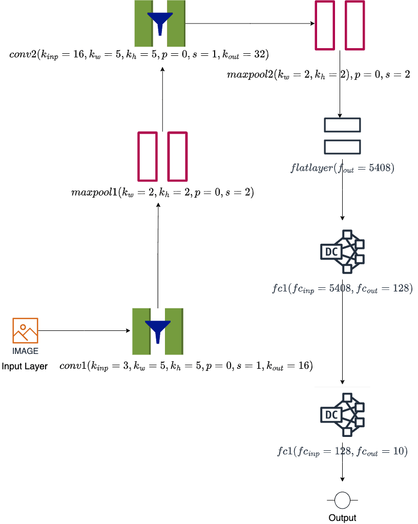
This network takes input as an RGB square image with three channels having width = height = 64.

We pass this image bitmap with three input channels to the first convolution layer, conv1, with kernel_size=(5, 5), stride=1, and padding=0, giving 16 output channels. Then, we pass it to a max pooling layer, maxpool1, with kernel_size=(2, 2) and stride=2, thereby keeping the output channels = 16.

Similarly, there’s a second convolution layer, conv2, with kernel_size=(5, 5) stride=1, and padding=2. This gives a feature map with 32 output channels.

Next, we’ve got the second max pool layer, maxpool2, with the same parameters as maxpool1. We process this feature map in the flat layer by flattening and converting it to a one-dimensional tensor. Then, we have two fully connected layers, fc1, with 128 neurons, and fc2, with 10 neurons (one for each class).

4.2. CNN Parameter Table

Let’s compute spatial dimensions and trainable parameter count of each layer in our example CNN:

Layer Name

Hyper Parameters

Input Dimensions

Output Dimensions

Learnable Parameter Count

conv1

inp=3, out=16, k=(5, 5), s=1, p=0

(64, 64, 3)

(60, 60, 16)

1216

maxpool1

w=(2,2), p=0, s=2

(60, 60, 16)

(30, 30, 16)

conv2

inp=16, out=32, k=(5, 5), s=1, p=0

(30, 30, 16)

(26, 26, 32)

12832

maxpool2

w=(2,2), p=0, s=2

(26, 26, 32)

(13, 13, 32)

flatlayer

none

(13, 13, 32)

5408

fc1

inp=5408, out=128

5408

128

692352

fc2

inp=128, out =10

128

1290

The total trainable parameter count is 707690.

5. PyTorch

Now, we’ll show how to compute the number in PyTorch.

5.1. Setup

First, let’s set up a virtual environment. We can use the pyenv or virtualenv tools to create it. After activating it, we need to install the following libraries:

torch
numpy

5.2. Libraries

Let’s load the necessary modules:

import torch
import torch.nn as nn
import torch.nn.functional as F

5.3. CNN Model

Here’s our CNN model:

class MySimpleCNN(nn.Module):
    def __init__(self, image_size, image_channels, conv_inp_feat, conv_out_feat, 
                   kernel_size, pool_size, fc1_out, num_classes):
        super(MySimpleCNN, self).__init__()
        self.conv1 = nn.Conv2d(image_channels, conv_inp_feat, kernel_size=kernel_size)
        self.pool = nn.MaxPool2d(pool_size, pool_size)
        self.conv2 = nn.Conv2d(conv_inp_feat, conv_out_feat, kernel_size=kernel_size)

        # Flatten layer
        with torch.no_grad():
            dummy_input = torch.randn(1, image_channels, image_size[0], image_size[1])
            x = self.pool(F.relu(self.conv1(dummy_input)))
            x = self.pool(F.relu(self.conv2(x)))
            flattened_size = x.view(1, -1).size(1)

        self.fc1 = nn.Linear(flattened_size, fc1_out)
        self.fc2 = nn.Linear(fc1_out, num_classes)

    def forward(self, x):
        x1 = self.pool(torch.relu(self.conv1(x)))
        x2 = self.pool(torch.relu(self.conv2(x1)))
        x3 = torch.flatten(x2, 1)
        x4 = F.relu(self.fc1(x3))
        y_cap = self.fc2(x4)
        return y_cap

It’s the same network as before.

5.4. CNN Model Parameter

With all the groundwork, we’re ready to calculate the parameters of our sample CNN. A trainable parameter is one whose value gets updated (learned) as the model trains on the training data (via backpropagation).

The most straightforward way to get the total parameter count of our PyTorch models is using the PyTorch function numel():

def count_parameters(model):
    return sum(p.numel() for p in model.parameters() if p.requires_grad)

Let’s now use it to calculate the parameter count:

image_size = (64, 64)
image_channels = 3
conv_inp_feat = 16
conv_out_feat = 32
kernel_size = 5
pool_size = 2
fc1_out = 128
num_classes = 10

device = torch.device("cuda" if torch.cuda.is_available() else "cpu")
model = MySimpleCNN(image_size, image_channels, conv_inp_feat, conv_out_feat,
                      kernel_size, pool_size, fc1_out, num_classes).to(device)

print(f"Total Trainable Parameters via {count_parameters.__name__}(): {count_parameters(model)}")

Here’s the output:

Total Trainable Parameters via count_parameters(): 707690

Compared to Resnet50 (50 layers) with $\approx 25.6$ million parameters, our network (8 layers) has $\approx 0.7$ million.

6. Conclusion

In this article, we studied how to determine the parameter count for a CNN.

Knowing this number helps us estimate model capacity, compute requirements, resource usage, and overall risk of overfitting. Furthermore, parameter calculation is a stepping stone for model compression, layer pruning, and quantization.

Persistence

REST

Security