1. Introduction
In this tutorial, we’ll explore explainable AI (XAI), why it’s important, and the different methods used to make AI more understandable.
We’ll also discuss two popular XAI methods, SHAP and LIME, with examples. By the end, we’ll have a clearer idea of how XAI makes AI decisions more transparent.
2. What Is Explainable AI?
Explainable AI (XAI) refers to techniques and tools designed to make AI systems more interpretable by humans. Many AI models, especially complex ones like neural networks, are often considered “black boxes” because they provide results without explaining how they reached those conclusions.
XAI helps break down this complexity, offering insights into how AI systems make decisions. This transparency is crucial for trust, regulatory compliance, and identifying potential biases in AI systems.
When we understand how AI systems work, we’re more likely to trust their decisions, especially in critical areas like healthcare or finance. Additionally, regulatory bodies often require transparency in AI systems to ensure fairness and accountability. Finally, understanding how AI systems make decisions can help identify and mitigate potential biases that may be present in the data or algorithms used to train models.
3. Types of Explanation Methods
We can categorize explanation methods based on agnosticity, scope, and data type. These criteria help distinguish how each technique works and where to apply it effectively.
3.1. Specificity
Specificity refers to whether the method can be applied to any model (i.e., is model-agnostic) or only works with specific types of models (model-specific).
Model-agnostic methods can be applied to any machine-learning model regardless of its underlying architecture. Examples include:
- SHAP (Shapley Additive Explanations) – Provides consistent feature importance scores based on cooperative game theory
- LIME (Local Interpretable Model-agnostic Explanations) – Builds a simpler model to approximate local predictions for any classifier or regressor
- Partial Dependence Plots – Shows the relationship between a feature and the prediction outcome for any model
Model-specific methods are tailored for specific model types and cannot be used for others. Some examples are:
- Tree SHAP – A variant of SHAP specifically for tree-based models like decision trees or random forests
- Feature importance for decision trees – Measures the importance of features by how much they reduce the error in tree-based models
- Attention mechanisms – We primarily use them in neural networks, especially in natural language processing (NLP) models, to show which input parts the model focuses on when making predictions
3.2. Explainable AI Methods Based on Scope
Explainability methods can also differ in scope, depending on whether they explain the entire model (global) or individual predictions (local).
Global methods explain how the entire model behaves across all data points. Some global methods are:
- Feature importance – Measures the overall importance of each feature in making predictions
- Partial Dependence Plots – Explains how each feature impacts predictions globally by showing marginal effects on model output
Local methods explain individual predictions, providing insights into why the model made a particular decision for one instance. Some examples include:
- LIME – Locally approximates a complex model with a simpler, interpretable model around the instance of interest
- SHAP – Assigns importance scores to each feature for a specific instance, explaining that particular prediction
3.3. Explainable AI Methods Based on Data Type
Different XAI methods are better suited for specific data types, such as tabular data, images, or text.
Tabular-data methods explain models trained on structured, tabular data:
- SHAP and LIME work well for tabular data by showing feature importance or local approximations
- Feature importance plots and partial dependence plots are common techniques for explaining tabular models
Image-data methods visualize which parts of an image were most influential in the model’s prediction:
- Grad-CAM – Visualizes the important regions in an image by highlighting areas that most contribute to the model’s output
- Saliency maps – Show which pixels or regions of an image are most important to the prediction
Text-data methods explain models trained on natural language:
- Attention mechanisms – Show which words or phrases the model “attends” to when making predictions
- LIME for text – Highlights important words or phrases that influenced the model’s decision for a particular instance
4. Examples
Two of the most widely used Explainable AI methods are SHAP (Shapley Additive Explanations) and LIME (Local Interpretable Model-agnostic Explanations).
Both methods offer feature-level explanations but approach the problem in different ways.
4.1. SHAP
SHAP is based on game theory. It computes consistent feature importance by assigning each feature a “Shapley value,” indicating how much each feature contributes to a prediction and ensuring that the sum of all feature contributions equals the model’s output.
SHAP can work globally (for the entire model) and locally (for specific predictions). In this example, we’ll use SHAP as a global method to determine the feature importance. For that purpose, we’ll use the California housing dataset from the sklearn library to predict house values based on some features.
Here’s a Python example using SHAP with a random forest regressor:
import shap
import pandas as pd
from sklearn.datasets import fetch_california_housing
from sklearn.model_selection import train_test_split
from sklearn.ensemble import RandomForestRegressor

# load the California housing dataset
housing = fetch_california_housing()
X = pd.DataFrame(housing.data, columns=housing.feature_names)
y = pd.Series(housing.target)

# split data into train and test sets
X_train, X_test, y_train, y_test = train_test_split(X, y, test_size=0.3, random_state=0)

# train a Random Forest Regressor
model = RandomForestRegressor(n_estimators=100, random_state=42)
model.fit(X_train, y_train)

# use SHAP to explain the model's predictions
explainer = shap.TreeExplainer(model)
shap_values = explainer.shap_values(X_test)

# create a summary plot
shap.summary_plot(shap_values, X_test)
Summary plot:
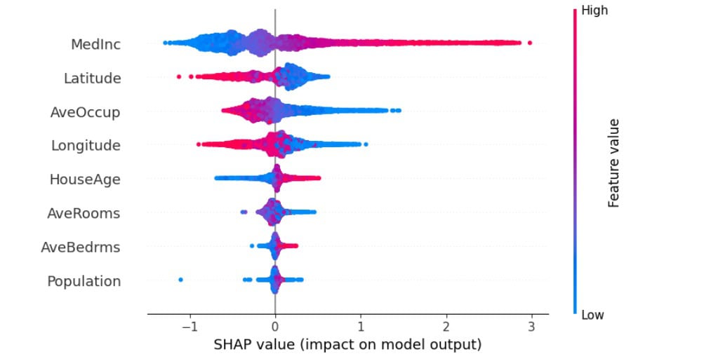
In the image above, features are sorted by the sum of the SHAP value magnitudes across all samples. The color represents the feature value (red for high, blue for low).
For example, the MedInc feature impacts the total model most, and its higher values correlate with higher model output. This means that a high MedInc increases the predicted home price.
Note that SHAP values can be negative, which means they decrease the predicted house price. For example, the Latitude feature is mostly red on the negative SHAP value side. This means that the correlation between Latitude and SHAP values is negative, so a high Latitude value lowers the predicted price.
4.2. LIME
LIME works by approximating the complex model with a simpler interpretable model (e.g., linear regression or decision tree) around a specific instance. LIME generates new synthetic data points around the instance, and then a simple model is used to explain how the features of that particular instance contribute to the prediction.
Here’s a Python example using LIME with a random forest classifier:
import lime
import lime.lime_tabular
from sklearn.datasets import load_iris
from sklearn.ensemble import RandomForestClassifier
from sklearn.model_selection import train_test_split

# load the dataset
data = load_iris()
X = data.data
y = data.target

# train-test split
X_train, X_test, y_train, y_test = train_test_split(X, y, test_size=0.3, random_state=42)

# train a RandomForest model
model = RandomForestClassifier(n_estimators=100, random_state=42)
model.fit(X_train, y_train)

# explain model predictions with LIME
explainer = lime.lime_tabular.LimeTabularExplainer(X_train, feature_names=data.feature_names, class_names=data.target_names, mode='classification')
explanation = explainer.explain_instance(X_test[0], model.predict_proba)

# display explanation
explanation.show_in_notebook()
We used LIME as a local method with the Iris dataset to explain the prediction of the first sample in the test data set:
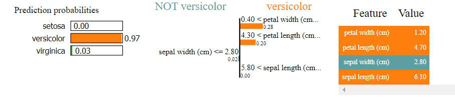
Our data set has three target classes: setosa, versicolor, and virginica. The model predicts that the first sample is versicolor with 97% probability. This prediction is based on features petal width (because it’s 1.2, which is higher than 0.4) and petal length (because it’s 4.7, higher than 4.3).
5. Conclusion
In this article, we discussed what explainable AI (XAI) is and why it’s important for AI transparency and trust. By breaking down complex models into understandable components, XAI offers insights into how models make decisions, ensuring accountability and mitigating biases.
We categorized various XAI methods based on their model-agnostic or model-specific nature, their scope (global or local), and the type of data they work with.
We also provided practical examples using SHAP and LIME. These methods can produce global and local explanations, enhancing our ability to interpret AI models in real-world applications.