What’s the Difference Between a Turing Machine and a Finite-State Machine?

1. Introduction

Turing machine (TM) and finite state machine (FSM) are foundational concepts of computational theory. Understanding them is crucial for understanding how modern computers process and compute data.

In this tutorial, we’ll explain how these abstract computation models work and learn about their history and principles. We’ll also compare them in detail and discuss their differences.

2. Turing Machine

Alan Turing introduced the Turing machine in 1936 as an abstract computation model. It’s a theoretical device that models computation as manipulating symbols on an infinite tape based on predefined rules.

There are many variants of Turing machines, such as non-deterministic, multi-tape multi-head, or one-way tape models. In this tutorial, we’ll focus on the standard, deterministic TM. It consists of a single head and a single infinite two-way tape.

2.1. Components

A TM consists of a moving head and a theoretical bidirectional infinite tape that acts as the machine’s memory and contains cells. Each cell can contain a single symbol from a specified and finite alphabet. The head can move left and right over the tape to read and write symbols:

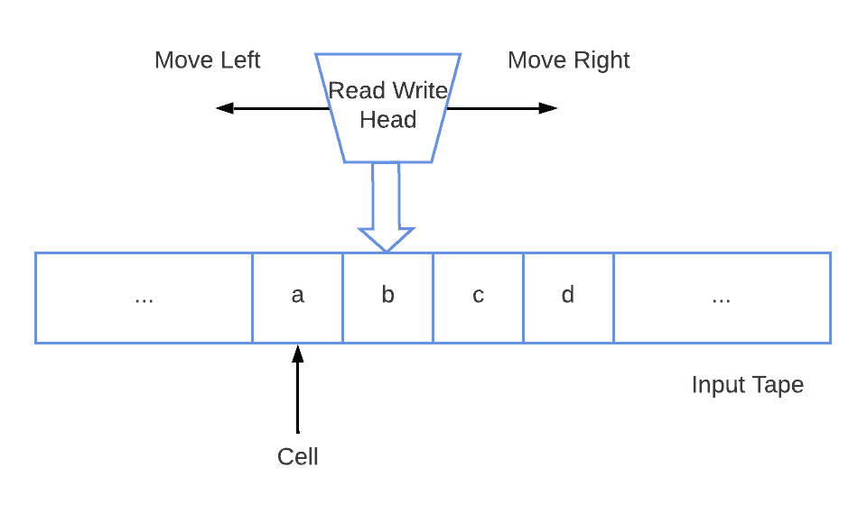Turing Machine The head moves in steps. In each step, it’s located above a single cell and executes operations according to the transition function.

The transition function defines how the head moves and what it writes in a cell based on the symbol it reads and the machine’s state. It also specifies how the machine transitions from one state to another depending on the read symbols.

2.1. Transition Function and Workflow

Formally, the transition function $\delta$ of a Turing machine is defined as:

$[\delta : Q \times \Gamma \to Q \times \Gamma \times \{L, R\}]$

The notation is as follows:

– The set of states that the Turing machine can be in
$F \subseteq Q$ – The set of final states
$\Gamma$ – The set of symbols that can be written on the tape
, where:
- $q \in Q$ – The current state of the machine
- $\gamma \in \Gamma$ – The symbol being read by the head
- $q' \in Q$ – The new state the machine will transition to
- $\gamma' \in \Gamma$ – The symbol that will be written in the current cell of the tape
- \item $d \in \{L, R\}$ – The direction in which the head will move: – left and – right

So, the whole process works deterministic****ally, as there’s a strictly defined instruction for each combination of state and symbol.

A TM works until the tape content is exhausted or no transition exists for the current combination of the state and head. When it halts, a TM accepts the input if it stops in a final accepting state. Otherwise, it rejects the input. However, a TM may run infinitely if it never reaches a state-head pair that causes it to stop.

3. Finite-State Machines

A finite state machine (FSM) is a basic computation model representing systems in a limited number of states.

Further, a finite state machine can move between the states only in response to external operants. In contrast to a TM, an FSM has no memory other than recording the current state. Thus, it’s more straightforward but less powerful in terms of processing.

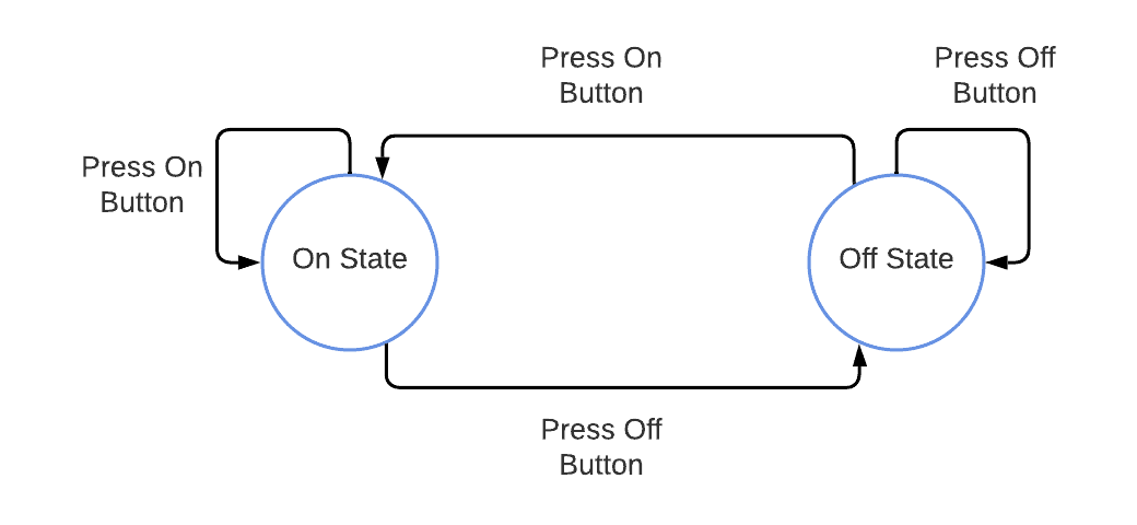
A simple example of a finite state machine would be a keyboard containing only two buttons, “On” and “Off.” For example, we can assume that it manages the power of some device, like a server or TV:

Final-state machine example

3.1. Transition Function

The transition function of an FSM is:

$[\delta : Q \times \Sigma\to Q]$

The notation is as follows:

– The set of all possible states of the FSM
$F \subseteq Q$ – The set of final states
$\Sigma$ – The set of input symbols, also known as the input alphabet
, where:
- $q \in Q$ – The current state of the FSM
- $a \in \Sigma$ – The input symbol being processed
- $q' \in Q$ – The state to which the FSM transitions after processing the input

3.2. Workflow

At the beginning of the workflow, the FSM is in the designated initial state. It starts receiving input.

The transition function considers the current state and determines the next for each input symbol. The process is deterministic, meaning each combination of state and input has exactly one transition path.

Further, an FSM continues reading input and switching to different states until it reads all input symbols. The final state can represent different outcomes, such as accepting or rejecting inputs, completing a task, or terminating the program. This deterministic behavior makes FSMs useful tools in systems engineering and computer science.

It’s important to note that there are other variants of FSMs, including non-deterministic FSMs or models with more complex components. For any non-deterministic finite-state machine, we can construct an equivalent deterministic one.

3.3. Finite Automata vs. Finite State Machines

The terms finite automata (FA) and finite state machines are often used interchangeably, which is usually correct. However, in some contexts, there are slight differences between the two terms.

A finite automaton is a more formalized and theoretical mathematical model. The theory of formal languages and automation mainly uses FA for tasks related to analyzing and designing languages, such as syntax analyzers.

On the other hand, FSMs tend to be practical tools for describing the operative logic of devices and control systems and are less formal than FA. We can represent a finite state machine in various ways, for example, using state diagrams or code.

4. Comparison

4.1. Memory

The Turing machine uses infinite tape as its memory, so it can store unlimited data during execution.

On the other hand, an FSM has no memory. As a result, a finite state machine depends only on its actual state and the current input symbol (disregarding the previous input symbols and states).

The limited memory makes FSM a less complex and less powerful model than the Turing machine.

4.2. Computational Complexity

A TM is theoretically capable of simulating any algorithm on any input. Its transition function’s complexity is due to using the tape’s content. Thus, the machine can consider not only its current state but also the symbols recorded on the tape to determine the next step. This complexity allows a Turing machine to solve a broader range of computational problems, as it can handle dynamic data throughout the process.

In contrast, an FSM depends only on the current state and input symbol. It doesn’t reference any external or stored data. Therefore, an FSM is a more predictable model, and its transitions are clearly described by the immediate context, making it suitable for systems with well-defined and limited requirements.

4.4. States

Turing machines and FSMs have one initial state and one or more final states.

The final states inform us about the outcome. The result describes whether the execution succeeds and whether the input is accepted.

4.5. Construction

The Turing machine consists of infinite two-way tape and a head that can read and write symbols on it. Each cell on the tape can store a single symbol, so the Turing machine can manipulate the data on the tape during processing.

In contrast, an FSM doesn’t have a tape and a head that can write on it. It operates only on a limited set of states and transitions between them. The only “data” FSM stores is its current state, as the transition depends on the state and received input symbol.

4.6. Usage and Applications

⁤The Turing machine is mainly used in theoretical contexts. Further, it defines the concept of an algorithm and explores the limits of computation.

Its complexity and infinite memory make it helpful in algorithm simulation. So, researchers use it in theoretical proofs and the analysis of undecidable problems and various algorithms.

On the other hand, FSMs are widely used in practical fields, such as digital circuit design and automatic control.

Due to its simplicity and deterministic nature, an FSM is ideal for modeling simple systems. Such systems need to go through specific sequences of states. Examples include communication protocols, device controllers, or character behavior in computer games.

4.7. Summary

Here is a quick summary of the differences and similarities between Turing machines and finite-state machines:

Feature

Turing Machine

Finite State Machine (FSM)

Memory

Infinite tape serving as memory

No memory

Computational complexity

High, can process any algorithm

Unable to solve problems requiring memory

Applications

Theoretical computation models, algorithm simulation

Modeling simple systems, formal language analysis, digital circuits

Transition function

Complex, may depend on tape content

Simple, deterministic, depends only on the current state and input

Problem-solving capability

Can solve problems with infinite data sets

Limited to problems solvable in finite time with a limited data set

States

One initial state and one or more final states

Construction

Consists of a head that moves alongside the tape

No memory tape

Example applications

Algorithm simulation, theoretical proofs, halting problem

Syntax analysis of languages, logic circuits, automatic control

For every FSM, we can construct a TM that will work the same, but the converse doesn’t hold.

5. Conclusion

In this article, we explained and compared two fundamental concepts of computation theory: Turing machines and finite-state machines.

The Turing machine can simulate any algorithm thanks to its unlimited memory and power. Therefore, it’s a great tool for researching theoretical systems.

In contrast, FSM is a simple tool with a limited set of states. Because it’s finite and less complex, it effectively models practical solutions like digital circuits.

Persistence

REST

Security