Beta Distribution | Baeldung中文网

1. Introduction

In this tutorial, we’ll explain the mathematics and intuition behind the family of Beta distributions in statistics and analyze their shapes.

2. Intuition

Let’s say we flip a fair coin 10 times and bet on tails with our friend. Since heads and tails are equally likely each time, our win probability in each toss is 1/2.

Then, the number of tails in 10 flips follows the binomial distribution centered at (1/2) * 10 = 5:

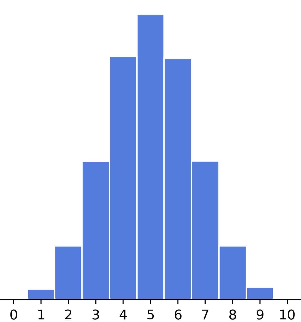
From there, we can derive how much we can expect to win in this game and decide how much money to bet.

However, what if the question is reversed? We flip a coin 10 times and get eight wins. We may be delighted with the financial gain, but our friend, not so much, so we get accused of using a biased coin.

To resolve the dispute, we must determine the coin’s inherent probability of landing on its tails in a random toss. This is precisely what Beta distributions can do.

The Beta distribution with parameters $\boldsymbol{a}$ and $\boldsymbol{b}$ shows how much each $\boldsymbol{x \in [0, 1]}$ is likely as the success probability, given that there were $\boldsymbol{a-1}$ successful and $\boldsymbol{b-1}$ unsuccessful trials.

3. Density

Beta-distributed random variables are defined over [0, 1] and have the following density:

$[f(x; a, b) = C x^{a-1} (1-x)^{b-1} \quad 0 \leq x \leq 1 \text{ and } a,b > 0]$

The constant ensures that the cumulative distribution function is 1 for x=1 :

$[1 = \int_{0}^{1}f(x; a, b)dx = C \int_{0}^{1} x^{a-1} (1-x)^{b-1} dx = C \cdot B(a, b) \implies C = \frac{1}{B(a, b)}]$

where B(a, b) is the beta function:

$[B(a, b) = \frac{\Gamma(a) \Gamma(b)}{\Gamma(a + b)} \qquad \Gamma(u) = \int_{0}^{\infty}t^{u-1}e^{-t}dt]$

Therefore, the density is:

$[f(x; a, b) = \frac{1}{B(a, b)}x^{a-1}(1-x)^{b-1}]$

3.1. Why Is There -1?

Essentially, the -1 in the exponents comes from the -1 in the integrand of the Gamma function.

We can try to find some intuition in it using the measure theory.

The CDF of the Beta distribution with parameters and is:

$[F(t; a, b) = \int_{0}^{t}f(x; a, b)dx = \int_{0}^{t}\frac{1}{B(a, b)}x^{a-1}(1-x)^{b-1}dx]$

Let’s move -1 to the denominator:

$[F(t; a, b) = \int_{0}^{t}\frac{1}{B(a, b)}\frac{x^{a}}{x}\frac{(1-x)^{b}}{1-x}dx = \int_{0}^{t}\frac{1}{B(a, b)}x^{a}(1-x)^{b}\frac{dx}{x(1-x)}]$

Now, we have:

$[\frac{dx}{x(1-x)} = d\left( \log \frac{x}{1-x} \right) = d\mu(x) \text{ for } \mu(x) = \log\frac{x}{1-x}]$

As a result, we can transform the CDF to:

$[\int_{0}^{t}\frac{1}{B(a, b)}g(x; a, b)d\mu(x) \quad g(x)=x^{a}(1-x)^{b}]$

where the density doesn’t have -1 in the exponents, and and are the numbers of successful and unsuccessful trials.

Intuitively, if we weigh each probability with the logarithm of the corresponding odds ratio, we can use this interpretation of and . In more technical terms, the density is defined with respect to the measure $\mu$ .

3.2. Non-Integer Parameters

The parameters and can be non-integers. However, the intuitive explanation was that a-1 and b-1 denote the numbers of successful and unsuccessful trials (or and if we use the measure $\mu$ ). How do we interpret a fractional or ?

Sometimes, the boundary between success and failure is clear-cut. For example, an experiment (a trial) can have several goals. Achieving some while failing at others constitutes partial success. To allow for this nuanced approach to evaluation, we use non-integers and .

4. Properties

Let’s now check some properties of this distribution family.

4.1. Mean

The mean of a Beta distribution with parameters and is:

$[\int_{0}^{1}xf(x; a, b) dx= \frac{1}{B(a, b)}\int_{0}^{1}x^{a}(1-x)^{b-1}dx = \frac{B(a+1, b)}{B(a, b)}]$

To simplify the expression, we’ll write B(a, b) using the Gamma function $\Gamma$ and note that $\Gamma(u+1) = u \Gamma(u)$ :

$[\frac{B(a+1, b)}{B(a, b)} = \frac{\frac{\Gamma(a+1) \Gamma(b)}{\Gamma(a+b+1)}}{\frac{\Gamma(a)\Gamma(b)}{\Gamma(a+b)}} = \frac{\frac{a \Gamma(a)}{(a+b)\Gamma(a+b)}}{\frac{\Gamma(a)}{\Gamma(a+b)}} = \frac{a}{a+b}]$

If $\boldsymbol{a=b}$ , the mean is 1/2. If $\boldsymbol{a>b}$ , the distribution’s center is shifted to the right and to the left if $\boldsymbol{a<b}$ .

This has an intuitive explanation. If there are many successful outcomes, it makes sense to believe that the probability of success is higher and vice versa.

4.2. Variance

We can similarly compute the variance:

$[\frac{ab}{(a+b)^2 (a+b+1)}]$

The larger and , the smaller the variance. That is also intuitive. The more experiments we conduct, the more we know about the success probability, so the distribution we use as its model should be less variable.

4.3. Skewness

The skewness of a distribution quantifies its deviation from symmetry. In the case of a beta distribution with shape parameters and , the skewness is:

$[\frac{2(b-a)\sqrt{a+b+1}}{(a+b+2)\sqrt{ab}}]$

So, for , the distribution is symmetric, right-skewed for , and left-skewed for .

This also has an intuitive explanation. If the number of successes equals the number of unsuccessful trials, there are no grounds to believe the true success probability is more likely to be > 1/2 than < 1/2, and vice versa. A symmetric distribution fits this assertion.

By the same logic, if a>b , successful trials are a majority, so it’s reasonable to believe that the true success probability is > 1/2. The right model for this assertion is a distribution centered around a value > 1/2. However, the remaining tail stretching to 0 makes the distribution left-skewed. The converse holds for a<b .

4.4. Kurtosis

The formula for the excess kurtosis is a bit more complex:

$[\frac{6\left((a-b)^2(a+b+1) - ab(a+b+2) \right)}{ab(a+b+2)(a+b+3)}]$

Negative values indicate tails lighter than those of the normal distribution, and positive values indicate heavier tails. The exact effect on the shape depends on the values of other moments (that are, in turn, defined by and ).

4.5. Mode

The mode of a distribution is its most likely value, i.e., the value with the highest density.

So, to compute it, we need to find $x \in [0, 1]$ that maximizes the density f(x; a, b) . Setting the first derivative of to zero and solving for , we get that the mode is:

$[\frac{a-1}{a+b-2}]$

For a symmetric distribution, a=b , and the mode is equal to the mean:

$[\frac{a-1}{a+a-2}=\frac{a-1}{2(a-1)}=\frac{1}{2}]$

5. Shapes

Depending on the values of and , the Beta density can take many shapes.

5.1. Symmetric Shapes

Symmetric shapes have a=b , and we differentiate between three cases:

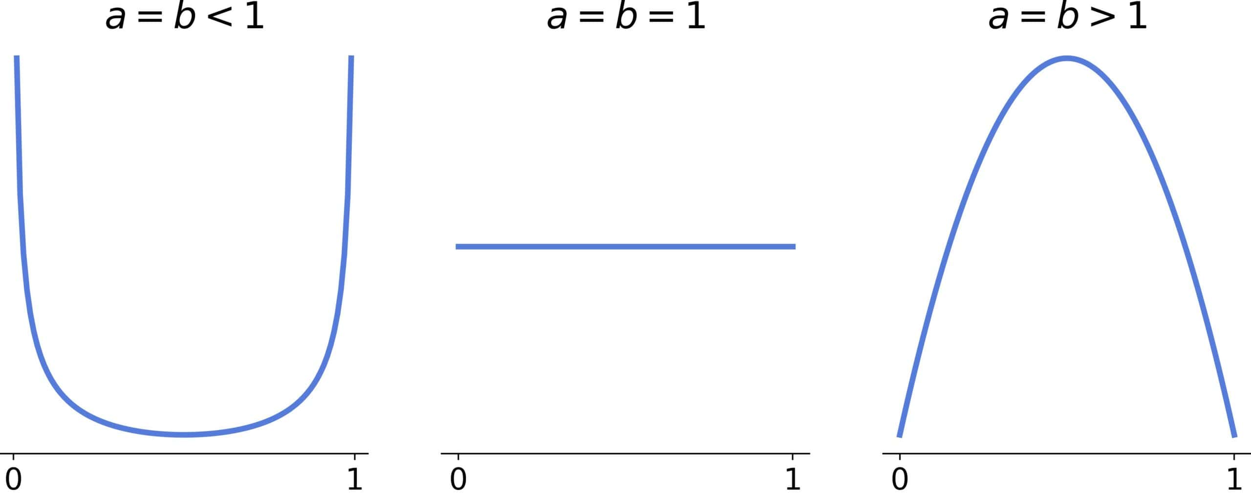
The special case a=b=1 corresponds to the uniform distribution.

If a, b < 1 , the distribution is U-shaped, and if a, b > 1 , it’s bell-shaped and approaches the normal distribution as and increase:

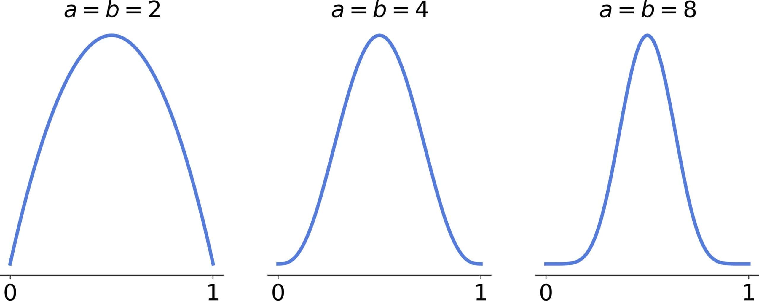
There will be two inflection points if a, b > 2 .

5.2. Asymmetric Shapes

For asymmetric shapes, b>a corresponds to right-skewed, and a<b to left-skewed distributions.

If both a, b < 1 , the distribution will be convex, approaching an L-shape (reversed or not) as the larger parameter approaches 1:

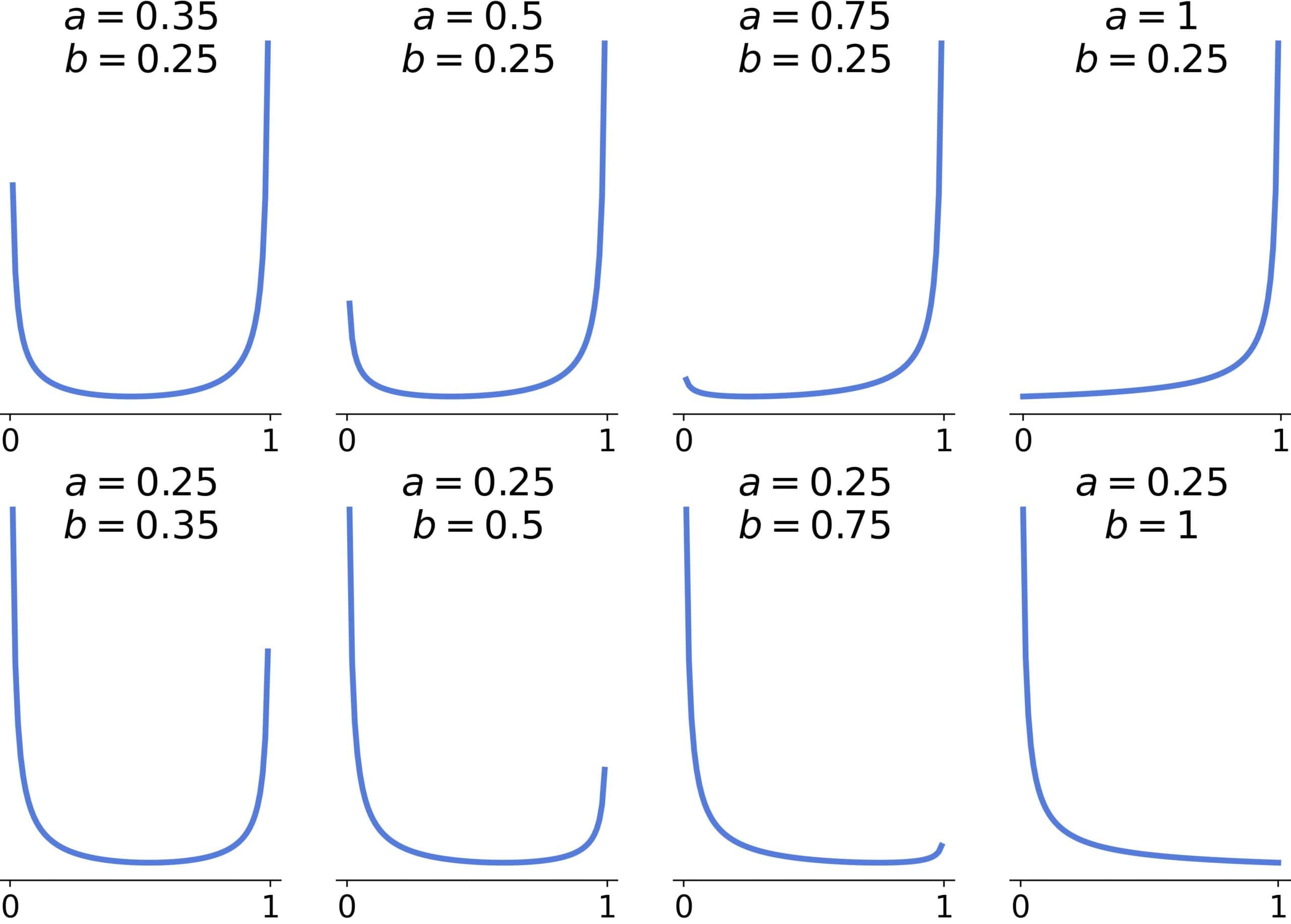
If a, b > 1 , the distribution will be unimodal, and the tail heaviness will decrease as the parameters’ difference grows. There will be one inflection point if one parameter is >2 and two inflection points if both are >2:

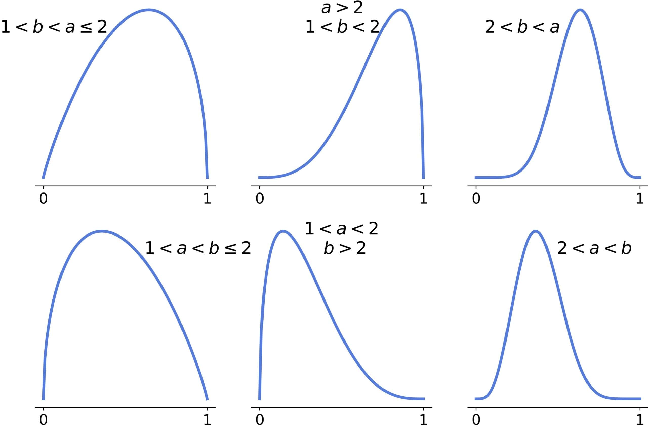
If a < 1 and b > 1 or if a > 1 and b < 1 , the shape will be convex or with one inflection point:

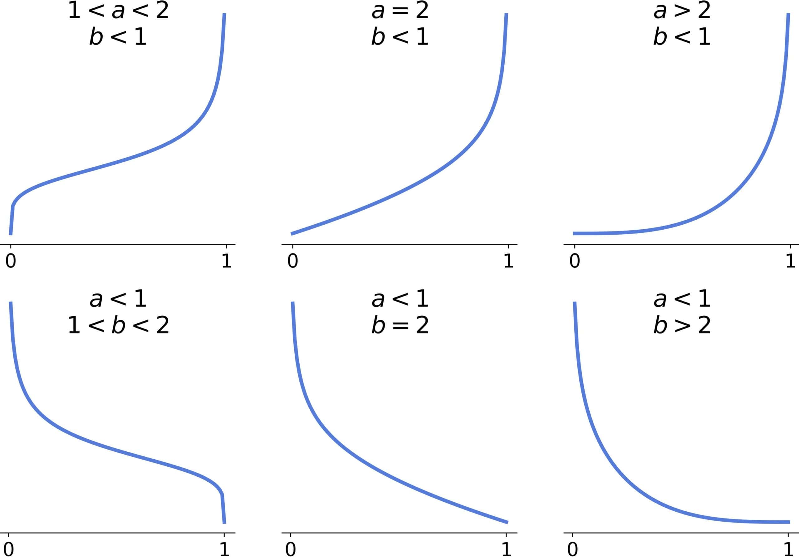
The inflection point will be there if 1< a, b < 2 .

The last remaining cases are a=1, b > 1 and a>1, b=1 :

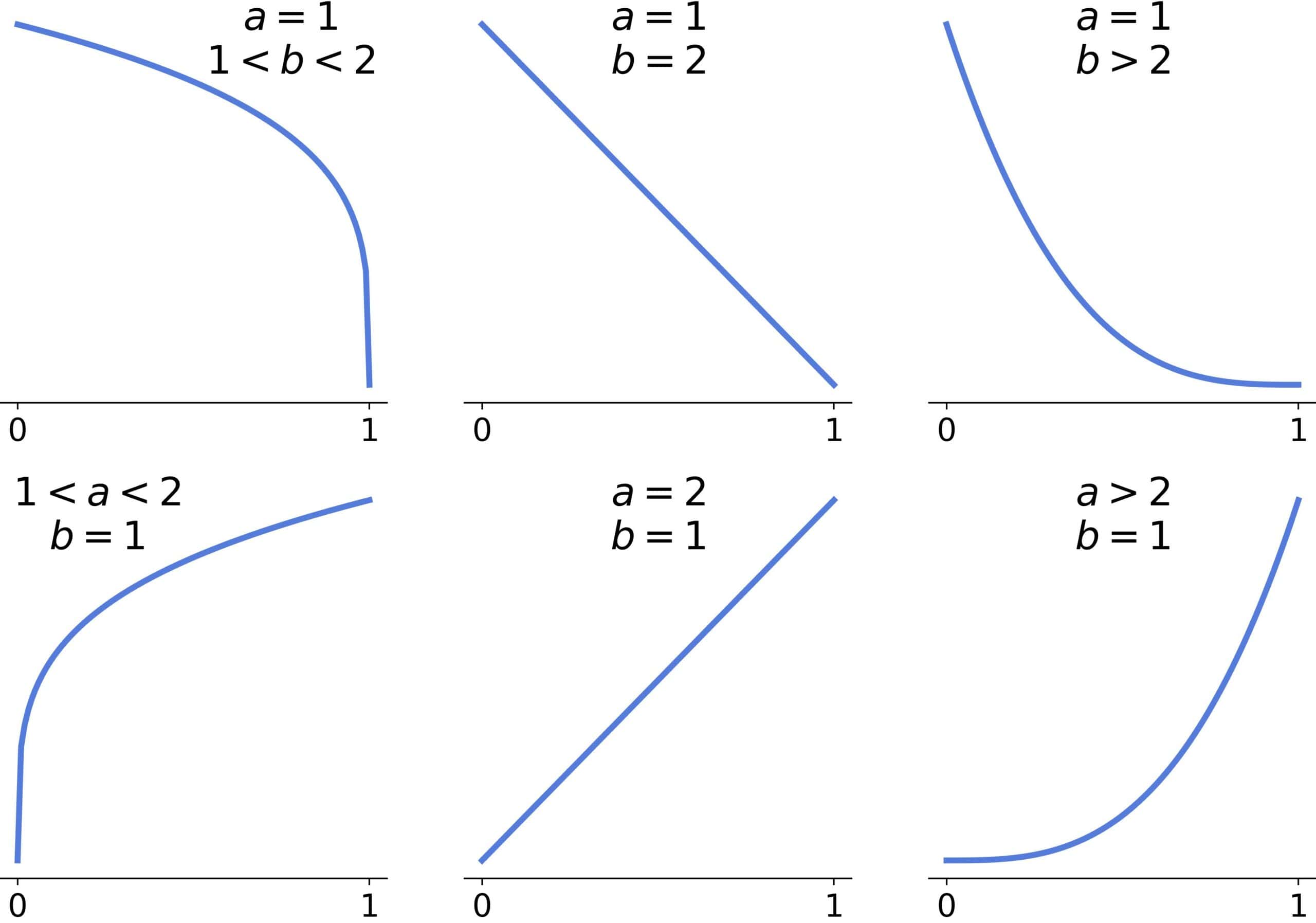
We have a straight line if the larger parameter equals two, a concave curve if it’s <2, and a convex one if it’s >2.

6. Conclusion

In this article, we discussed the family of Beta distributions in statistics. These distributions are defined over [0, 1] and can take many shapes, making them suitable for modeling normalized quantities (such as probabilities).

Persistence

REST

Security