Why Does the L1 Norm Enforce Sparsity in Models?

1. Introduction

We often find that the use of L1-norm forces sparsity in the model. In a Machine Learning context, this involves setting certain feature coefficients to zero. This selects only the most relevant features that contribute significantly to the output. But why does L1-norm work in these scenarios?

In this tutorial, we’ll define the L1-norm and then show examples of how it is used for sparse models.

2. How Does the L1-Norm Ensure Sparsity?

Let’s start with the simple definition of the L1-norm. Then, we’ll move on to how it works for optimization problems.

2.1. Definition

If we have a vector $\vec{\mathbf{x}} = (x_1, x_2, \ldots, x_n) \in \mathbb{R}^n$ the L1-norm is the sum of the absolute values of its components.

$\begin{equation} [ \|\vec{\mathbf{x}}\|_1 = \sum_{i=1}^{n} |x_i| ] \end{equation}$

Let’s start building our intuition with the vector $\vec{\mathbf{x}} = (1, \epsilon) \in \mathbb{R}^2$ , with $\epsilon > 0$ , but very small. If we apply a regularization $\eta \ll \epsilon$ to the first coordinate, x_1 , the L1-norms becomes

(1) $\begin{equation*} \|\vec{\mathbf{x}}\|_1 = (1 - \eta) + \epsilon \end{equation*}$

And if we apply to x_2 we obtain

(2) $\begin{equation*} \|\vec{\mathbf{x}}\|_1 = 1 +( \epsilon - \eta) \end{equation*}$

We can see that even though the first coordinate is much larger than the second one, the applied regularization is the same.

To compare, let’s take a look at the definition of the L2-norm:

$\begin{equation} [ \|\mathbf{x}\|_2 = \sqrt{\sum_{i=1}^n x_i^2} ] \end{equation}$

And if we apply the L2-norm to the first coordinate x_1 :

(3) $\begin{equation*} \|\vec{\mathbf{x}}\|_2^2 = 1 - 2\eta + \eta^2 + \epsilon^2 \end{equation*}$

and if we apply only to the second component x_2 we have

(4) $\begin{equation*} \|\vec{\mathbf{x}}\|_2^2 = 1 - 2\eta \epsilon + \eta^2 + \epsilon^2 \end{equation*}$

So we see that the L2-norm applies a much smaller regularization to the smaller component x_2 , since $2\eta \epsilon \ll 2\eta$ .

We can now elaborate on our first argument to build our intuition. The L2-norm will hardly set anything to zero since the regularization is reduced as we approach a smaller value for any coordinate. But the L1-norm will always result in a penalty $\eta$ that even though $|x_1| \gg |x_2|$ .

2.2. Optimization Framework

Now let’s see in a more realistic scenario for a constrained minimization problem for $\vec{\mathbf{\beta}} = (\beta_{1}, \beta_{2})$

$\begin{equation} [ \min_{\vec{\mathbf{\beta}} } \|y - X \vec{\mathbf{\beta}} \|_2^2 + \lambda \|\vec{\mathbf{\beta}} \|_1 \textrm{, s.t. } \|\vec{\mathbf{\beta}} \|_1 \leq 1 ] \end{equation}$

We can visualize the feasible region defined by this constraint, where the L1-norm of $\vec{\mathbf{\beta}}$ can’t be greater than one:

l1 norm feasible region

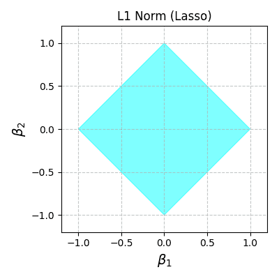
Now, let’s consider a general group of least square loss functions, as shown in the red contours. We highlight the contour that touches the diamond in cyan:

lasso with loss

With the L1-norm, the cost function represented by the red and cyan ellipses minimizes along the boundaries of the diamond until it reaches a vertex (spike).

We can see that the loss function touches the feasible region at one of the spikes where $\beta_1 = 0$ and $\beta_2 = 1$ . By setting $\beta_2$ to zero we found a solution that only requires one component, so we can observe sparsity.

We might think that this is a coincidence for a specific example. But for different loss functions, especially in high dimensions, it’s more likely that they will touch the diamond in one corner. We only need to use the appropriate scaling for the constraint by adjusting $\lambda$ . To make things clearer, let’s look at how the L2-norm works.

2.3. A Counter-Example: L2-Norm

Let’s take a look at the L2 norm to make things more evident. If we consider the L1 and L2 norms and the groups of loss functions, we have:

l1 l2 norm loss

The red, green, and brown points represent unconstrained least square solutions for three functions. The contours around these points are gradient descent contours with only scaling adjustments. In the center, we have the same diamond as before but also a circle that represents the feasible region for the L2-norm.

The curves in cyan represent all the loss functions for each problem intersecting the L1-norm feasible diamond-shaped region. We do the same for the L2-norm but with black curves that touch the circle centered at ( 0,0 ).

If we analyze the black ellipse and circles, we see that none of the curves touches a sparse point ( $\beta_1=0$ or $\beta_2=0$ ). This illustrates how hard it is for the L2 norm to promote sparsity, given its smooth shape.

But if we look at the cyan curves we see that the intersection points are either exactly on one of the axis or at least much closer to the axis. With this geometric intuition, we can see why L1-norm promotes sparsity.

2.4. The Gradient of L1-norm

As a final argument, let’s consider the derivatives of the L1 and L2 norms:

derivatives

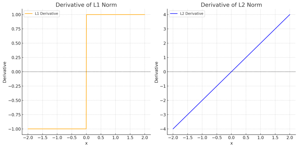
We can see that the L1-norm has a derivative equal to for positive values of and for negative values of . While the derivative of the L2-norm is , increasing linearly with in a smooth way. So we see that the L1 derivative has a constant absolute value and a discontinuity at x=0 . During the optimization process, this constant derivative applies a steady force pulling coefficients toward zero. Once a coefficient gets close to zero, the optimization naturally “snaps” it to exactly zero because of the abrupt shift at the origin.

3. Polynomial Example

Let’s consider now a polynomial example. We add noise to the data points from the function

(5) $\begin{equation*} y = 3x^3 - 2x^2 + 0.5 + \delta \end{equation*}$

Then, we approximate this with a 5th-degree polynomial using both Lasso (L1-norm) and Ridge (L2-norm) regressions. For Lasso, we obtain the coefficients [ 0, 0, 1.81, -0.2, 0.16] and for Ridge [ 1.21, -1.97, 2.87, 0.007, 0.001] . We can also take a look at the prediction for each regression:

lasso and ridge

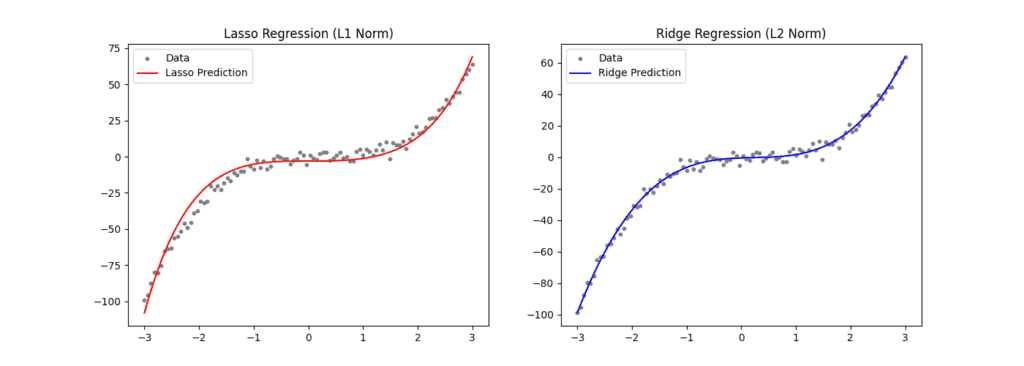
As expected, we see some sparsity in the Lasso regression coefficients. The first two coefficients of the polynomial are exactly zero. This means we have a simpler model that has less chance of overfitting than the L2-norm-based model since we have a model that didn’t learn less important features.

And we have that without compromising the quality of the regression. A quick qualitative look at both results shows that the data points are well approximated.

We should always consider using an L1-norm penalty for feature selection. It reduces the complexity of the model by setting irrelevant features to zero, while still learning important features.

4. Conclusion

In this article, we discussed why the L1-norm is used for sparse models. Its geometrical properties ensure that we keep only the most essential features. Every other less relevant feature will be set to zero and ignored. In that way, we end up with a model with good generalization capability.

Persistence

REST

Security