Understanding Regularization in a Neural Network

1. Introduction

In neural networks overfitting leads to poor generalization, meaning the model performs well on the data it has seen but fails to deliver accurate predictions on new, unseen data. As the size and complexity of neural networks grow, the risk of overfitting increases significantly.

This is where regularization comes into play. Regularization techniques are essential in controlling the complexity of neural networks and preventing them from fitting the noise in the data.

In this tutorial, we’ll explore various regularization methods used in neural networks, explaining how they work, and their necessity.

2. What Is Regularization?

Regularization is a set of techniques in machine learning that aim to improve a model’s ability to generalize from its training data to unseen data. In the context of neural networks, regularization helps prevent the model from overfitting, a common problem where the network becomes too good at predicting the training data but struggles to perform well on new data.

The main goal of regularization is to strike a balance between a model that is too simple (which could underfit the data and fail to capture important relationships) and one that is too complex (which overfits and captures irrelevant noise). Regularization enhances the model’s ability to generalize, ensuring it performs well on new data it will encounter.

3. How Regularization Works?

Regularization typically adds a penalty term to the model’s loss function. The loss function is what the model tries to minimize during training, as it measures the difference between the model’s predictions and the actual values. Regularization modifies this loss function by adding a term, which penalizes larger or more complex models.

For example, let’s say the original loss function is , and it measures how well the model fits the training data. With regularization, the loss function becomes:

(1) $\begin{equation*} L_{regularized} = L + \lambda \cdot \text{Penalty}L_{regularized} \end{equation*}$

In this equation, $L_{regularized}$ is the new loss function that incorporates regularization. is the original loss function, such as mean squared error or cross-entropy. $\lambda$ is the regularization parameter, which controls how much regularization is applied. A higher $\lambda$ increases the penalty, making the model simpler. Penalty refers to the added regularization term. This term varies depending on the type of regularization method used.

The penalty term discourages the model from learning overly complex solutions by either shrinking the model parameters or limiting their growth, leading to a more generalized solution. Different types of regularization apply different kinds of penalties, such as forcing some weights to be zero or reducing the magnitude of all weights.

3.1. Example

If we consider a neural network with two weights w_1 = 1.5 and w_2 = 0.5 . The original loss (mean squared error) without regularization is L=0.5. With L_2 regularization, the loss becomes, $L_{L2}= L + \lambda \sum w_i^2$ .

Using $\lamda = 0.01$ , the regularized loss is, $L_2 = 0.5+0.01 \cdot (1.52+0.52)=0.5+0.01\cdot(2.25+0.25)=0.525$ .

Here, L_2 regularization adds a penalty of 0.025 to the original loss. Over many iterations, this prevents overfitting by discouraging large weight values.

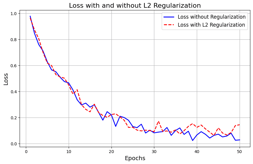
As training continues, the loss decreases, but without regularization, overfitting can occur, harming generalization. The red dashed line shows L2 regularization, which slightly increases the loss initially but helps prevent overfitting by keeping the weights smaller, improving generalization:

L2 Vs No regularization

4. Types of Regularization

These methods introduce additional constraints or penalties during training, making the model more robust and better able to generalize to new data. In this section, we will cover the most commonly used regularization techniques.

4.1. L1 Regularization (Lasso)

L1 regularization, also known as Lasso (Least Absolute Shrinkage and Selection Operator), works by adding the absolute values of the model’s weights to the loss function. This method encourages sparsity in the model, meaning that many weights will become zero during training. As a result, the model uses only a subset of the most important features, which can lead to simpler, more interpretable models.

The loss function for L_1 regularization is:

(2) $\begin{equation*} L_{L1}= L + \lambda \sum |w_i|L_{L1} \end{equation*}$

In the above equation, is the original loss (e.g., mean squared error or cross-entropy), $\lambda$ is the regularization parameter, which controls the strength of the penalty and $\w_{i}$ represents the individual weights of the model.

In L_1 regularization, the regularization term adds the sum of the absolute values of all weights to the loss function. As the model trains, less important weights are pushed to zero, effectively removing them from the model.

This sparsity is beneficial in high-dimensional datasets where many features may be irrelevant. L_1 regularization can be thought of as a feature selection method, automatically determining which features are most important by reducing the others to zero.

4.2. L2 Regularization (Ridge)

L_2 regularization, also known as Ridge regression, adds the squared values of the weights to the loss function, encouraging smaller but non-zero weights. Unlike , which tends to push some weights to exactly zero, regularization penalizes large weights more heavily, resulting in a smoother distribution of weight values.

The loss function for L_2 regularization is:

(3) $\begin{equation*} L_{L2}= L + \lambda \sum w_i^2L_{L2} \end{equation*}$

Here, is the original loss, $\lambda$ is the regularization parameter and $\w_{i}$ represents the individual weights.

In L_2 regularization the regularization term adds the sum of the squares of the weights to the loss function. This approach discourages large weights by penalizing them more as they grow, which prevents the model from becoming too complex.

L_2 regularization tends to result in models with many small weights rather than a few large weights. This helps smooth the learning process, making the model less sensitive to small fluctuations in the training data, leading to better generalization.

5. Other Regularization Techniques

Beyond L_1 and L_2 regularization, several other techniques have proven highly effective in preventing overfitting in neural networks. These methods go beyond simply adding penalties to the loss function, instead introducing innovative strategies that directly affect the training process or modify the network’s structure.

5.1. Dropout

Dropout is one of the most popular and effective regularization techniques for deep neural networks. It was introduced by Geoffrey Hinton et al. in 2012. Dropout involves randomly “dropping out” a fraction of the neurons in a layer during each training iteration. This prevents the network from becoming too reliant on any single neuron and forces it to learn more robust features.

The key idea behind dropout is to break the co-adaptation of neurons, where certain neurons become dependent on each other. By randomly dropping neurons during training, dropout simulates training many different, smaller networks and helps the network become less sensitive to individual neurons.

5.2. Early Stopping

Early stopping is a regularization technique that monitors the model’s performance on a validation set during training, and it stops training once the validation error starts to increase. This prevents the model from overfitting to the training data by ensuring that training is halted before the model learns noise and irrelevant details.

During training, the error on the training set usually decreases with each iteration. Still, after a certain point, the model may begin to overfit, leading to an increase in the validation error. Early stopping stops training when the validation performance no longer improves, preventing overfitting.

5.3. Batch Normalization

Batch Normalization is a technique that was initially introduced to help stabilize and accelerate the training of deep networks. But it also serves as an effective regularizer. The idea is to normalize the inputs to each layer so that they have a mean of zero and a standard deviation of one. This normalization process is applied across each mini-batch of training data, ensuring that each layer receives inputs on a consistent scale.

Batch normalization reduces internal covariate shift, which helps the model learn more efficiently and reduces the risk of overfitting.

5.4. Data Augmentation

Data Augmentation is a technique used to expand the training dataset artificially. It does so by creating modified versions of the original data. This is particularly common in image-based tasks. Operations like rotating, flipping, cropping, or adjusting brightness can generate new training samples. These samples provide additional data for the model to learn from.

By increasing the diversity of training data, data augmentation helps the model generalize better. The model learns to recognize patterns under various conditions. This reduces the risk of overfitting the original dataset and improves unseen data performance.

6. Choosing the Right Regularization Technique

Selecting the appropriate regularization technique for a neural network depends on several factors, including the dataset’s size, the model’s complexity, and the problem at hand. A table summarizing these cases:

Characteristic or Case

Regularization Technique

Small dataset

L2 regularization or Dropout

Large dataset

Batch normalization and early stopping

Deep Networks

Dropout and Batch Normalization

Shallow Networks

L2 or L1 regularization

High-Dimensional Data

L1 regularization

Image Data

Data augmentation and Dropout

7. Conclusion

Regularization is a critical concept in building effective neural networks. This is especially true when dealing with complex models prone to overfitting. By introducing constraints such as L1 and L2 penalties, Dropout, and techniques like Batch Normalization, regularization helps. Data Augmentation also contributes to improving the model’s ability to generalize to unseen data.

Persistence

REST

Security